Project 2 - Rankine cycle Simulator

AIM: To understand the Rankine Cycle and calcualte performance factors and plot the graphs for temp.vs entropy, enthalpy vs entropy.

OBJECTIVE:

• Create a Rankine Cycle Simulator using MATLAB.
• Calculate the state points of the Rankine Cycle based on the inputs.
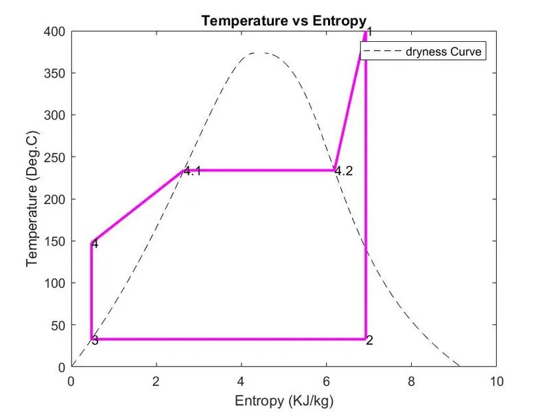
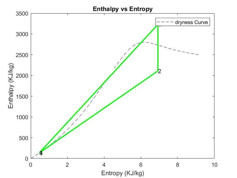
• Plot the corresponding T-s and h-s plots for the given set of inputs. Title and axes labels are a must, while legends could be used if necessary.

THEORY:

Rankine Cycle: The Rankine cycle is an idealized thermodynamic cycle describing the process by which certain heat engines, such as steam turbines or reciprocating steam engines, allow mechanical work to be extracted from a fluid as it moves between a heat source and heat sink.

Heat energy is supplied to the system via a boiler where the working fluid (typically water) is converted to a high-pressure gaseous state (steam) in order to turn a turbine. After passing over the turbine the fluid is allowed to condense back into a liquid state as waste heat energy is rejected before being returned to boiler, completing the cycle. Friction
losses throughout the system are often neglected for the purpose of simplifying calculations as such losses are usually much less significant than thermodynamic losses, especially in larger systems.

Sample output of a Basic Rankine cycle simulator:

• Type:Basic Rankine-

The above Rankine cycle figure contains four different processes which are as follows:

1. 1-2 = In process 1-2 dry saturated vapor expands through a turbine generating power. This decreases the temperature and pressure of the vapor and some condensation may occur.[Isentropic Expansion]
2. 2-3 = In process 2-3 wet vapor enters a condenser, where it is condensed at constant pressure to become saturated liquid.[Heat rejection at constant pressure]
3. 3-4 = In process 3-4 fluid is pumped from low to high pressure.[Isentropic compression]
4. 4-1 = In process 4-1 high-pressure liquid enters the boiler, where it is heated at constant pressure by an external heat source to become a dry saturated vapor.[Heat addition at constant pressure]

CODE LOGIC:

Here we dividided code into small parts to explain it breifly.

Part 1:

%Rankine cycle simulator program
clear all
close all
clc

%Displaying each state in the command window
disp('1-2 is Isentropic Expansion in the Turbine')
disp('2-3 is Const Pressure Heat Rejection by the Condensor')
disp('3-4 is Isentropic Compression in the Pump')
disp('4-1 is Const Pressure Heat Addition by the Boiler')
fprintf('\n')

%Input parameters
p1 = input('Enter the pressure at turbine inlet(in bar)= ');
t1 = input('Enter the temperature at turbine inlet(in degree(celcius)= ');
p2 = input('Enter the pressure at turbine outlet(in bar)= ');
fprintf('\n')

• Here we are dispalying the state points by using 'disp' command and asked for the input parameters p1,p2,t1.

Part 2:

% To get importants formulas

Tsat_P1 = XSteam('Tsat_p', p1);
hf_1 = XSteam('hL_p', p1);
hg_1 = XSteam('hV_p', p1);
hfg_1 = hg_1 - hf_1;
sg_1 = XSteam('sV_p', p1);
sf_1 = XSteam('SL_p', p1);
sgf_1 = sg_1 - sf_1;


Tsat_P2 = XSteam('Tsat_p', p2);
hf_2 = XSteam('hL_p', p2);
hg_2 = XSteam('hV_p', p2);
hfg_2 = hg_2 - hf_2;
sg_2 = XSteam('sV_p', p2);
sf_2 = XSteam('SL_p', p2);
sfg_2 = sg_2 - sf_2;

• By using 'XSteam' we calculated the specific properties

Terminology:
Tsat = Saturation temperature.

hf,sf are specific enthalpy and entropy at Liquid state.

hg,sg are specific enthalpy and entropy at Vapour state.

hfg,sfg are terms during the change of state of matter(water).

Part 3:

% At point 1:

h1 = XSteam('h_pt', p1, t1);   
s1 = XSteam('s_pt', p1, t1);

% At point 2:

s2 = s1;
x2 = (s2-sf_2)/sfg_2;
h2 = hf_2 + x2*(hfg_2);
t2=Tsat_P2;

%At point 3:

p3 = p2;
v3 = XSteam('vL_p', p3); 
t3 = Tsat_P2;    
h3 = hf_2;       
s3 = sf_2;


% At point 4:

p4 = p1;
s4 = s3 ;   
Wp = v3 * (p4 - p3)*100; 
h4 = Wp + h3; 
cpL= XSteam('CpL_p', p1);
x = (sf_1-s4)/cpL;
t4 = Tsat_P1/exp(x);
sf4 = XSteam('sL_p',p4);
sg4 = XSteam('sV_p',p4);

• For State 1: Since we know the pressure and temperature at entry point (turbine), we calculated the enthalpy and entropy at state 1.
• For State 2: Since We know the pressure and entropy is constant(s2=s1), We calculated the drynes fraction and enthalpy values at state 2.
• For State 3: Here pressure is constant from state 2 to state 3 (p3=p2), we calulated volume, enthalpy and entropy by using 'XSteam' data at state 3.
• For State 4: Here (p4=p1), (s4=s3) due to constant entropy and calculated the specific heat at at liquid, Pump work and temperature. The entropy values at saturated vapour and liquid is calculated by using 'Xsteam' data.

Part 4:

% Calculating performance parameters.
Wt = h1 - h2; 

Wp = h4 - h3;

Wnet = Wt - Wp;

Qin = h1 - h4; 

thermal_efficiecy = (Wnet / Qin)*100;     

Wbr = Wp/Wt;

SSC = 3600 / Wnet;   

• Here we calculated the performance parameters like

1. Turbine work
2. Pump work
3. Net workdone
4. Heat input
5. Thermal Efficiency
6. Back work ratio
7. Specific steam consumption

Part 5:

% To display all the proprties in command window.

disp('                               RESULTS                    ')
disp('At state point 1                 ')                        
fprintf('P1 = %f Bar              \n', p1);          
fprintf('T1 = %f °C               \n', t1);
fprintf('H1 = %f kJ/kg            \n', h1); 
fprintf('S1 = %f kJ/kgK           \n\n', s1)

disp('At state point 2                '); 
fprintf('P2 = %f Bar              \n', p2)       
fprintf('T2 = %f °C               \n', t2)    
fprintf('H2 = %f kJ/kg            \n', h2)     
fprintf('S2 = %f kJ/kg            \n', s2)  
fprintf('X2 = %f \n\n', x2)  

disp('At state point 3                ');
fprintf('P3 = %f Bar              \n', p3)
fprintf('T3 = %f °C               \n', t3)
fprintf('H3 = %f kJ/kg            \n', h3)
fprintf('S3 = %f kJ/kgK           \n\n', s3)

disp('At state point 4               ');
fprintf('P4 = %f Bar             \n',p4)
fprintf('T4 = %f °C              \n',t4)
fprintf('H4 = %f KJ/kg          \n', h4)
fprintf('S4 = %f KJ/kgK         \n\n', s4)


fprintf('S.S.C is : %f kg/kWh     \n', SSC) 
fprintf('Turbine work = %f kJ/kg   \n', Wt)
fprintf('Pump work = %f kJ/kg     \n', Wp)
fprintf('Net Wok done = %f kJ/kg  \n', Wnet)
fprintf('Thermal efficiency = %f percent   \n',thermal_efficiecy )
fprintf('Back work ratio = %f      \n\n',Wbr)

• To display the all parameters in command window We used 'fprintf' command and 'disp' command to print and display the results in command window.

Part 6:

%Getting data to plot dryness fraction lines in the plot
temp = linspace(1,400,500);
for i = 1 : length(temp)
     H_L(i) = XSteam('hL_T', temp(i));
     H_V(i) = XSteam('hV_T', temp(i));
     S_L(i) = XSteam('sL_T', temp(i));
     S_V(i) = XSteam('sV_T', temp(i));
end

• Here we declared the Temperature values and calculated Enthalpy Entropy at Liquid & Vapour states to plot the Dryness Fraction Curve in the graphs.

Part 7:

% Plotting T vs S
figure(1)
%Plotting dryness fraction curve
plot(S_L, temp,'color','[0 0 0.3]','linestyle','--')
hold on
plot(S_V, temp,'color','[0 0 0.3]','linestyle','--')

%plotting cycle curve

plot([s1 s2],[t1,t2],'color','m','linewidth',2)
plot([s2 s3],[t2,t3],'color','m','linewidth',2)
plot([s3 s4],[t3,t4],'color','m','linewidth',2)
plot([s4 sf4],[t4,Tsat_P1],'color','m','linewidth',2)
plot([sf4 sg4],[Tsat_P1,Tsat_P1],'color','m','linewidth',2)
plot([sg4 s1],[Tsat_P1,t1],'color','m','linewidth',2)

%defining the figure
title('Temperature vs Entropy')
xlabel('Entropy (KJ/kg)')
ylabel('Temperature (Deg.C)')
legend('dryness Curve')


%defining state points
text(s1,t1,'1')
text(s2,t2,'2')
text(s3,t3,'3')
text(s4,t4,'4')
text(sf4,Tsat_P1,'4.1')
text(sg4,Tsat_P1,'4.2')

• First we plotted the dryness fraction curve for T vs S [ temperature vs entropy]
• And then plotted the Rankine cycle curve for T vs S by using all state points.
• We define properties like title,legend,xlabel,ylabel.
• And texted the numbers at each point.

Part 8:

%plotting H vs S
figure(2)
%plotting dryness fraction curve
plot(S_L, H_L,'color','[0 0 0.5]','linestyle','--')
hold on
plot(S_V, H_V,'color','[0 0 0.5]','linestyle','--')

%plotting cycle curve
plot([s1 s2], [h1 h2],'color','g','linewidth',2)
plot([s2 s3], [h2 h3],'color','g','linewidth',2)
plot([s3 s4], [h3 h4],'color','g','linewidth',2)
plot([s4 s1], [h4 h1],'color','g','linewidth',2)

%defining the figure
title('Enthalpy vs Entropy')
xlabel('Entropy (KJ/kg)')
ylabel('Enthalpy (KJ/kg)')
legend('dryness Curve')


%Defining state points in the plot
text(s1,h1,'1')
text(s2,h2,'2')
text(s3,h3,'3')
text(s4,h4,'4')

• First we plotted the dryness fraction curve for H vs S [ enthalpy vs entropy]
• And then plotted the Rankine cycle curve for H vs S by using all state points.
• We define properties like title,legend,xlabel,ylabel.
• And texted the numbers at each point.

MAIN CODE:

%Rankine cycle simulator program
clear all
close all
clc

%Displaying each state in the command window
disp('1-2 is Isentropic Expansion in the Turbine')
disp('2-3 is Const Pressure Heat Rejection by the Condensor')
disp('3-4 is Isentropic Compression in the Pump')
disp('4-1 is Const Pressure Heat Addition by the Boiler')
fprintf('\n')

%Input parameters
p1 = input('Enter the pressure at turbine inlet(in bar)= ');
t1 = input('Enter the temperature at turbine inlet(in degree(celcius)= ');
p2 = input('Enter the pressure at turbine outlet(in bar)= ');
fprintf('\n')


% To get importants formulas

Tsat_P1 = XSteam('Tsat_p', p1);
hf_1 = XSteam('hL_p', p1);
hg_1 = XSteam('hV_p', p1);
hfg_1 = hg_1 - hf_1;
sg_1 = XSteam('sV_p', p1);
sf_1 = XSteam('SL_p', p1);
sgf_1 = sg_1 - sf_1;


Tsat_P2 = XSteam('Tsat_p', p2);
hf_2 = XSteam('hL_p', p2);
hg_2 = XSteam('hV_p', p2);
hfg_2 = hg_2 - hf_2;
sg_2 = XSteam('sV_p', p2);
sf_2 = XSteam('SL_p', p2);
sfg_2 = sg_2 - sf_2;


% At point 1:

h1 = XSteam('h_pt', p1, t1);   
s1 = XSteam('s_pt', p1, t1);

% At point 2:

s2 = s1;
x2 = (s2-sf_2)/sfg_2;
h2 = hf_2 + x2*(hfg_2);
t2=Tsat_P2;

%At point 3:

p3 = p2;
v3 = XSteam('vL_p', p3); 
t3 = Tsat_P2;    
h3 = hf_2;       
s3 = sf_2;


% At point 4:

p4 = p1;
s4 = s3 ;   
Wp = v3 * (p4 - p3)*100; 
h4 = Wp + h3; 
cpL= XSteam('CpL_p', p1);
x = (sf_1-s4)/cpL;
t4 = Tsat_P1/exp(x);
sf4 = XSteam('sL_p',p4);
sg4 = XSteam('sV_p',p4);

% Calculating performance parameters.
Wt = h1 - h2; 

Wp = h4 - h3;

Wnet = Wt - Wp;

Qin = h1 - h4; 

thermal_efficiecy = (Wnet / Qin)*100;     

Wbr = Wp/Wt;

SSC = 3600 / Wnet;   

% To display all the proprties in command window.

disp('                               RESULTS                    ')
disp('At state point 1                 ')                        
fprintf('P1 = %f Bar              \n', p1);          
fprintf('T1 = %f °C               \n', t1);
fprintf('H1 = %f kJ/kg            \n', h1); 
fprintf('S1 = %f kJ/kgK           \n\n', s1)

disp('At state point 2                '); 
fprintf('P2 = %f Bar              \n', p2)       
fprintf('T2 = %f °C               \n', t2)    
fprintf('H2 = %f kJ/kg            \n', h2)     
fprintf('S2 = %f kJ/kg            \n', s2)  
fprintf('X2 = %f \n\n', x2)  

disp('At state point 3                ');
fprintf('P3 = %f Bar              \n', p3)
fprintf('T3 = %f °C               \n', t3)
fprintf('H3 = %f kJ/kg            \n', h3)
fprintf('S3 = %f kJ/kgK           \n\n', s3)

disp('At state point 4               ');
fprintf('P4 = %f Bar             \n',p4)
fprintf('T4 = %f °C              \n',t4)
fprintf('H4 = %f KJ/kg          \n', h4)
fprintf('S4 = %f KJ/kgK         \n\n', s4)


fprintf('S.S.C is : %f kg/kWh     \n', SSC) 
fprintf('Turbine work = %f kJ/kg   \n', Wt)
fprintf('Pump work = %f kJ/kg     \n', Wp)
fprintf('Net Wok done = %f kJ/kg  \n', Wnet)
fprintf('Thermal efficiency = %f percent   \n',thermal_efficiecy )
fprintf('Back work ratio = %f      \n\n',Wbr)

%Getting data to plot dryness fraction lines in the plot
temp = linspace(1,400,500);
for i = 1 : length(temp)
     H_L(i) = XSteam('hL_T', temp(i));
     H_V(i) = XSteam('hV_T', temp(i));
     S_L(i) = XSteam('sL_T', temp(i));
     S_V(i) = XSteam('sV_T', temp(i));
end

% Plotting T vs S
figure(1)
%Plotting dryness fraction curve
plot(S_L, temp,'color','[0 0 0.3]','linestyle','--')
hold on
plot(S_V, temp,'color','[0 0 0.3]','linestyle','--')

%plotting cycle curve

plot([s1 s2],[t1,t2],'color','m','linewidth',2)
plot([s2 s3],[t2,t3],'color','m','linewidth',2)
plot([s3 s4],[t3,t4],'color','m','linewidth',2)
plot([s4 sf4],[t4,Tsat_P1],'color','m','linewidth',2)
plot([sf4 sg4],[Tsat_P1,Tsat_P1],'color','m','linewidth',2)
plot([sg4 s1],[Tsat_P1,t1],'color','m','linewidth',2)

%defining the figure
title('Temperature vs Entropy')
xlabel('Entropy (KJ/kg)')
ylabel('Temperature (Deg.C)')
legend('dryness Curve')


%defining state points
text(s1,t1,'1')
text(s2,t2,'2')
text(s3,t3,'3')
text(s4,t4,'4')
text(sf4,Tsat_P1,'4.1')
text(sg4,Tsat_P1,'4.2')

%plotting H vs S
figure(2)
%plotting dryness fraction curve
plot(S_L, H_L,'color','[0 0 0.5]','linestyle','--')
hold on
plot(S_V, H_V,'color','[0 0 0.5]','linestyle','--')

%plotting cycle curve
plot([s1 s2], [h1 h2],'color','g','linewidth',2)
plot([s2 s3], [h2 h3],'color','g','linewidth',2)
plot([s3 s4], [h3 h4],'color','g','linewidth',2)
plot([s4 s1], [h4 h1],'color','g','linewidth',2)

%defining the figure
title('Enthalpy vs Entropy')
xlabel('Entropy (KJ/kg)')
ylabel('Enthalpy (KJ/kg)')
legend('dryness Curve')


%Defining state points in the plot
text(s1,h1,'1')
text(s2,h2,'2')
text(s3,h3,'3')
text(s4,h4,'4')

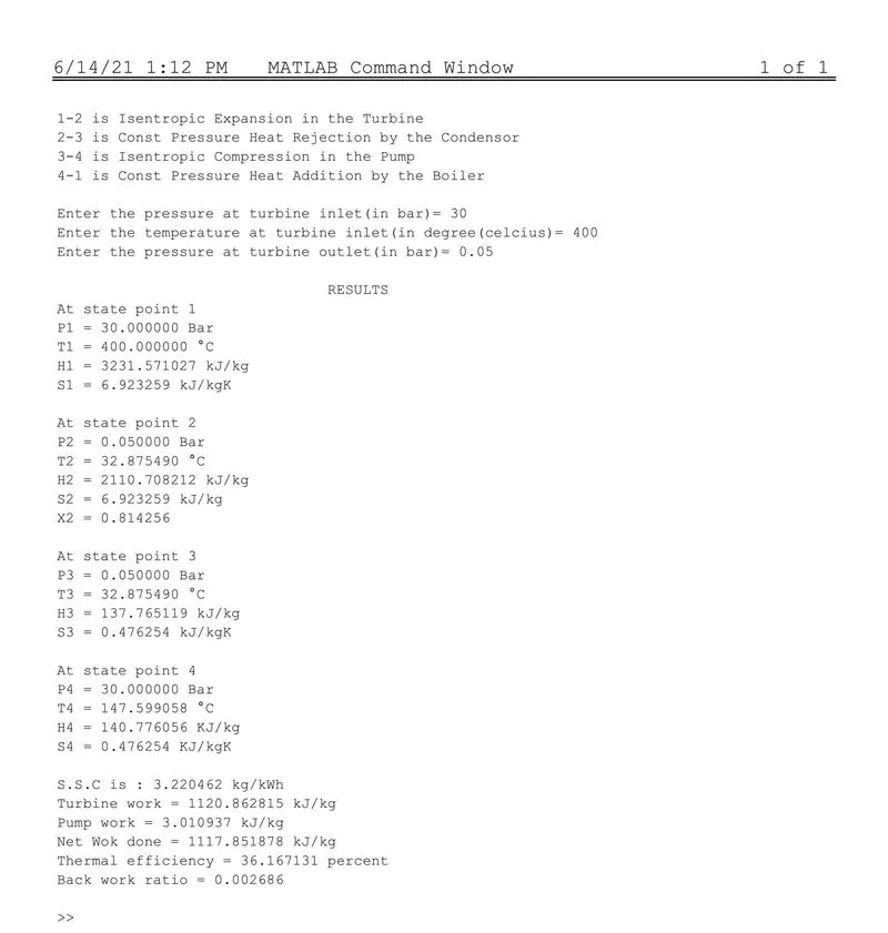
INPUTS:

• Turbine Inlet temperature = 400° C
• Turbine Inlet Pressure = 30 bars
• Turbine Outlet Pressure = 0.05 bars = Condenser Inlet Pressure

OUTPUTS:

• Result in command window

PLOTS:

T vs S H vs S

Results:

1. Net work output = 1117.851878 KJ/Kg
2. Back work ratio = 0.002686

CONCLUSION:

• Created a Rankine Cycle Simulator using MATLAB.
• Calculated the state points of the Rankine Cycle based on the inputs.
• Plotted the corresponding T-s and h-s plots for the given set of inputs and titled the plots and added legend to plots.
• Results are satisfactory.