Week 4.1 - Genetic Algorithm

Optimization is the process of selection from the set values for the imposed targets and the constraints.

It's processes handling many parameters, where its integrated with each other and affects ane another in all aspects.

Optimization techniques helps us to easily find a way to get the best out of very difficult selection of appropriate range of values for the defined targets and constraints.

Population Algorithm:- An algorithm that maintains an entire set of candidate solutions, and each solution corresponds to a unique point in the search space of the problem known as popupation based algorithm.

Some of the notable population based algorithm are as follows,
1)Genetic Algorithm
2)Differential Evolutoin
3)Partial Swarm Optimization

Genetic Algorithm:- It is a search based algorithms based on the concepts of natural selection and genetics. These are intelligent exploitation of random search provided with historical data to direct the search into the region of better performance in solution space. They are commonly used to generate high-quality solutions for optimization and search problems.

Here is the Program written below to optimise the stalagmite function.

clear all
close all
clc

%input space
x = linspace(0,0.6,150);
y = linspace(0,0.6,150);
%no. of iteration
num_case = 50;

%mesh by meshgrid
[xx,yy] = meshgrid(x,y);

for i = 1:length(x)
    for j = 1:length(y)
        
        input(1) = xx(i,j);
        input(2) = yy(i,j);
        input = [input(1),input(2)];
        f(i,j) = stalagmite1(input);
        
    end
end

figure(1)
surf(xx,yy,-f)
shading interp

%unbounded GA study
tic
for  i = 1:num_case
   
    [input,fopt(i)] = ga(@stalagmite1,2);
        xopt(i) = input(1);
        yopt(i) = input(2);
        
end
study_time1 = toc

figure(2)
subplot(2,1,1)
surf(x,y,-f)
shading interp
hold on
plot3(xopt,yopt,-fopt,'marker','o','markersize',5,'markerfacecolor','r')
title('Unbounded inputs')
subplot(2,1,2)
plot(-fopt)
xlabel('Iteration')
ylabel('Function maximum')

%bounded GA study
        
tic        
for i = 1:num_case
        
    [input,fopt(i)] = ga(@stalagmite1,2,[],[],[],[],[0;0],[0.4;0.4]);
                
    xopt(i) = input(1);
    yopt(i) = input(2);
                
end
study_time2 = toc

figure(3)
subplot(2,1,1)
surfc(x,y,-f)
shading interp
hold on
plot3(xopt,yopt,-fopt,'marker','o','markersize',5,'markerfacecolor','r')
title('Bounded inputs')
subplot(2,1,2)
plot(-fopt)
xlabel('Iteraion')
ylabel('Function maximum')


%bounded study with population size
options = optimoptions('ga');
options = optimoptions(options,'PopulationSize',270);

tic
for i = 1:num_case
    [input,fopt(i)] = ga(@stalagmite1,2,[],[],[],[],[0;0],[0.4;0.4],[],[],options);
    
    xopt(i) = input(1);
    yopt(i) = input(2);
    
end
study_time3 = toc;

figure(4)
subplot(2,1,1)
surfc(x,y,-f)
shading interp
hold on
plot3(xopt,yopt,-fopt,'marker','o','markersize',5,'markerfacecolor','r')
title('Bounded inputs')
subplot(2,1,2)
plot(-fopt)
xlabel('Iteration')
ylabel('Function maximum')

User defined function for evaluation of stalagmite equations...

function [f] = stalagmite1(input)
x = input(1);
y = input(2);

f1x = (sin((5.1*pi*x)+0.5))^6;
f1y = (sin((5.1*pi*y)+0.5))^6;
f2x = exp(-4*log(2)*(((x-0.0667)^2)/0.64));
f2y = exp(-4*log(2)*(((y-0.0667)^2)/0.64));


f = -(f1x*f1y*f2x*f2y);

end

In main program, I defined the search space with 2 variable x & y. For that, creates 1-dimensional array for x,y & use linspace command to provide 150 value between 0 to 0.6
After that I creates 2-dimensional array based on our 1-dimension array.

And then I used ‘for loop’, I define the Than I am creating an array called input(1), input(2) (row vectors) for each value of x,y and save these value in input.

After creating x,y variable(input variable),
as it does not define the search space for ‘ga’; ‘ga’ does not know its actual space and the value for x,y go beyond or below to 0.6 or 0.
For that I use num_cases=50, means I am going to run it 50 times.
Now to visualize my output, i use surface command(surfc), shading command(shading interp) is used to get smooth plot(without grid lines). in new figure window(figure1), I also use tic-toc command to calculate the time taken for evaluation. I use subplot command for multiple plotting.

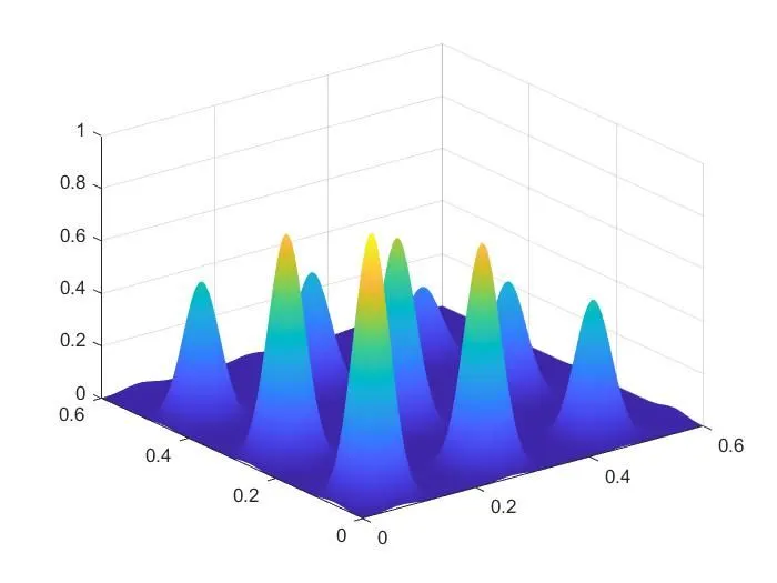
Here is the plotting output for general condition.

Here is the plotting output for Unbounded condition.

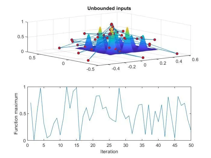
Here we can see the optimal values went outside the values of x and y resulting in falling away from stagalmite surface. So we failed to reach the global maxima in this case.

Here is the plotting output for Bounded condition.

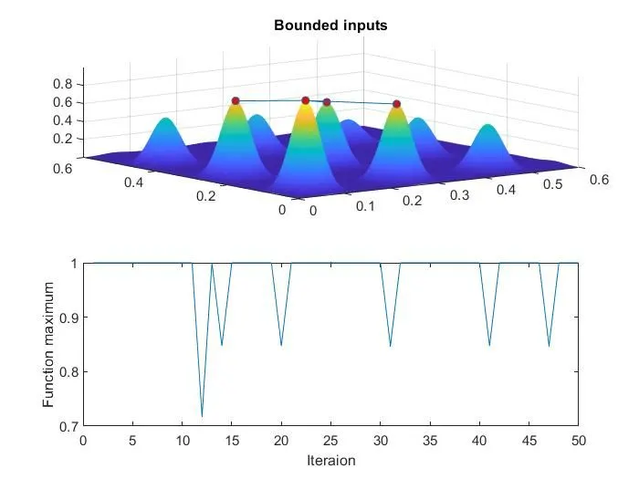
So, here the optimum values are within the limits it could not give us the exact maxima values.

Here is the plotting output for Bounded with Population size condition.

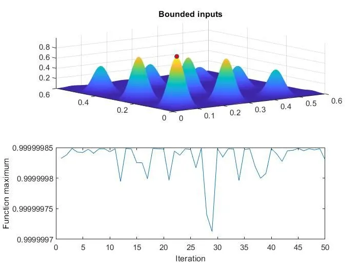
In this result we are successful to find out the correct maxima for the stalagmite function. So by increasing the initial population size of the 'ga' we can increase the accuracy of the algorithm.

Here is the Workspace output.

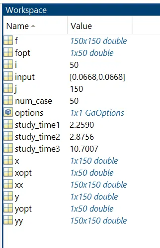
In workspace we can see that every array size is 150 as we had taken in llinspace.