Week 3 - Solving second order ODEs

ODE(Ordinary Differential Equation) is used to describe the transient behavior of a system. A pendulum at periodic motion is the best example of ODE.

Newtons second law of motion (The rate of change of linear momentum of a body is directly proportional to the external force applied on the body, and this change takes place always in the direction of the force applied.) defines the movement of Pendulum. When this law is written down, we get a Second order Ordinary Differential Equation that describes the position of the 'Bob'(point mass hanging at the end of string) with respect to Time, which is given below.

d2(θ)/dt2 + (b/m)(dθ/dt) + (g/l)sinθ = 0

where,
b=damping co-efficient,
m=mass of bob,
g=gravitational force,
l=length of string.

Here is the program given below to solve this second order ODE and plotting a graph for Angular velocity and Angular displacement of pendulum w.r.t. Time.

clear all
close all
clc

%inputs
b = 0.05;
g = 9.81; %in m/s^2
l = 1; %in metre
m = 1; %in kg

%initial condition 
theta_0 = [0;3];

%Time input
t_span = linspace(0,20,400);

%solving differential equation by using ode45 solver
[t,results] = ode45(@(t,theta) ode_function_pendulum(t,theta,b,g,l,m),t_span,theta_0);


figure(1)
hold on
plot(t,results(:,1),'color','r','linewidth',2)
plot(t,results(:,2),'color','b','linewidth',2)
xlabel('time in seconds')
ylabel('amplitude')
title('Damped harmonic motion of Pendulum')
legend('angular displacement','angular velocity')

x0 = 0;
y0 = 0;
displacement = results(:,1);
ct = 1;
for i = 1:length(displacement)
x1 = l*sin(displacement(i));
y1 = -l*cos(displacement(i));
figure(2)
plot([-2,2],[0,0],'linewidth',6,'color','r')
hold on
plot([x0,x1],[y0,y1],'linewidth',2,'color','b')
plot(x1,y1,'.','markersize',50,'color','g')
hold off
axis([-1.5 1.5 -1.2 1.2])
M(ct) = getframe(gcf);
ct = ct+1;
end

movie(M)
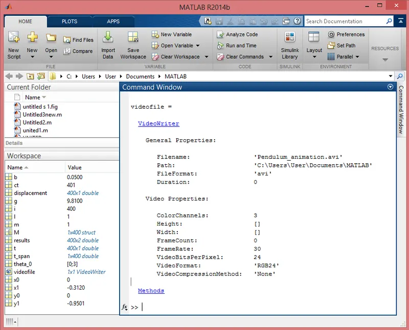
videofile = VideoWriter('Pendulum_animation.avi','uncompressed avi')
open(videofile)
writeVideo(videofile,M)
close(videofile)

Inputs is taken as per data given in the question, which is as follows,
damping co-efficient(b) = 0.05 kg
mass of bob(m) = 1 kg
gravitational force(g) = 9.81 m/s^2
length of string(l) = 1 m

Now I have taken initial condition as theta_0 = 0 radian angular displacement and 3 rad/sec angular velocity of pendulum.
and I have taken a span of time from 0 second to 20 second with 400 equal distrubution to gain a smooth curve for plotting of graph.

And then, ode45 syntax is used to solve the equation, but I have to describe a self defined function for that, which is given below...

function [derivation] = ode_function_pendulum(t,theta,b,g,l,m)

theta1 = theta(1); %displacement rep as an array
theta2 = theta(2); %Velocity rep as array

d_theta1_dt = theta2; %first differential
dtheta2_dt = ((-b/m)*theta2-((g/l)*sin(theta1))); %second differential

derivation = [d_theta1_dt; dtheta2_dt]; %combination of equation that is to be solved

end

Function named ode_function_pendulum firstly have to save in same path as the main program has been saved.

To solve second order differrential I had to break this equation in first differential and second differential equation, which gives the result as the Angular displacement and Angular Velocity in arrays.
These arrays are assign to variable called theta1 and theta2 respectively.

"plot" command is used to plot the graph of 'time v/s angular displacement and angular velocity, which I got by solving eqution and is named "results", in form of arrays. "hold on" cocmmand is also used to capture both output in a single graph page.
This graph is titled "Damped harmonic motion of Pendulum".

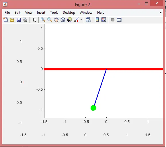
To pendulum animation, I defined one more plotting in which I took a frame of reference of -2 to 2 at x-axis and 0,0 at y-axis.
and then to create string if pendulum x0 to x1 point at x-axis and y0 to y1 point is used.
x1 is derived by using formula x1 = L1sinθ and y1 is derived by using formula y1 = -L1cosθ.

To create the bob of pendulum "plot" command is used but dot(.) is represented with markersize 50.

An animated video file is also created of this moving pendulum in harmonically way.
For which M(ct)=getframe(gcf) command is used to capture every frame and movie(M) to save the videofile in AVI.

After running this program, screenshot of output command page is given below...

A graph is plotted for Amplitude of Angular displacement and Angular Velocity with chsnge Time.

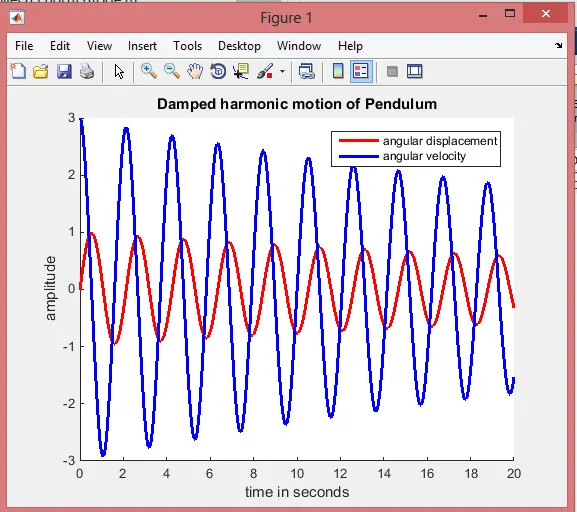
As we can see in this graph blue line is termed as Angular velocity and red line is as angular displacement.
Curve of angular displacement initiates from zero and, of angular velocity initiates from 3, as per our starting condition given.

Here also we can see that, due to damping in the system amplitude of velocity and displacement is decreasing with respect to Time.

Image of pendullum is shown below which obtained by plotting graph of figure 2.

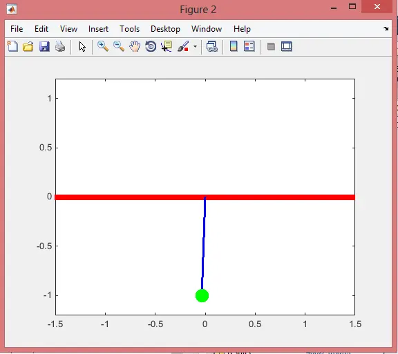
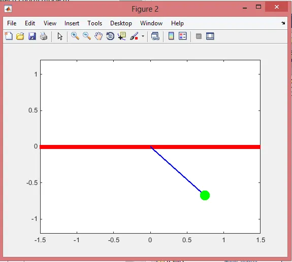
Animation snap is shown below regarding making of a video file.

An animated video file of this periodically moving pendulum is attached.

End.

(Sir, video file was so large which can not be uploaded, so I compressed it through video cpmpressor application, consequenced an water mark is being shown on my animated video and also name of that file is changed. So, I request you to ignore these two things.)