Challenge

Week 4.1 - Genetic Algorithm

AAsma Banu S16 Jul 2022

Aim: Is to Try to understand the concept of genetic algorithm by referring to varius sources before you attend this challenge. Look out for information regarding stalagmite function and ways to optimise it.

Write a code in MATLAB to optimise the stalagmite function and find the global maxima of the function.
Clearly expalin the concept of genetic algorithm in your own words and also explain the syntax for ga in MATLAB in your report.
Make sure that your code gives the same output, even if it is made to run several times.
Plot graphs for all 3 studies and for F maximum vs no. of iterations. Title and axes labels are a must, legends could be shown if necessary.

The presentation of your code will be taken into consideration while grading. Labeling sections of your code is appreciated.

Content expected in the report:

Step-wise explanation of your code.
Mention the errors while programming.
Steps taken to overcome those errors.
Screenshots showing errors thrown in command window.

Genetic algorithms (GA)

The genetic algorithm (GA) approach to optimisation is based upon the concept of survival of the fittest The GA emulates the processes of evolution and is therefore an evolutionary algorithm. In such a process the strongest elements become stronger while the weakest elements are eliminated.

The solution of an optimisation problem using the GA methodology involves a stochastic search of the solution space using strings of integers, known as chromosomes, which represent the parameters being optimised. Each integer within these chromosomes is known as a gene and, for these modelling applications, each gene has a decimal value between 0 and 9. It should be noted that this is not the traditional GA approach where genes are binary quantities. The advantage of the decimal representation for this type of application is that it allows a wider range of possible values in smaller chromosomes and is particularly suitable for both model and design optimisation.

An initial population of chromosomes is generated at random and these are decoded to obtain the corresponding parameters. These parameter values are then introduced into the system model. A simulation is run and results are obtained for each set of parameters within the population, using a measure of performance based on a cost function similar to that used in simulated annealing. When the cost values are all found, they are sorted into ascending order along with the corresponding chromosomes. As before, the smallest cost values are chosen as the best and are then subjected to operations involving reproduction, crossover and mutation.

The reproduction procedure involves retaining the best chromosomes (say 20 per cent) for the next population. The other chromosomes are replaced by new chromosomes formed through processes of crossover and mutation. This reproduction process is termed ‘rank-based selection’ and allows only the elite chromosomes to proceed to the next iteration. This method is therefore an elite genetic algorithm

Crossover is a process in which two chromosomes from the current generation (parent chromosomes) engage in a procedure in which some genes from one chromosome are interchanged with genes from the corresponding positions in the other. This process produces two new chromosomes (offspring) and the procedure is repeated until there are sufficient offspring to replace the 80 per cent of the present population that have the worst cost values.

Mutation involves selection, on a random basis, of a certain number of the genes in the current population and random alterations are then made to their values. This provides a random element within the GA search process so that more of the search space is considered.

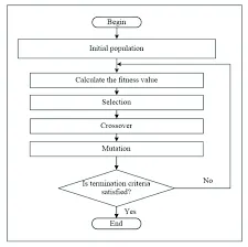
Once the chromosomes have been changed to form the new population they have to be evaluated, as were the previous generation. The whole procedure is then repeated for a predefined number of iterations (generations) to produce a final solution. This complete procedure is illustrated by the flow diagram of Figure

syntax for ga

x = ga(fun,nvars) :x= ga(fun,nvars) finds a local unconstrained minimum, x, to the objective function, fun. nvars is the dimension (number of design variables) of fun.
x = ga(fun,nvars,A,b):x= ga(fun,nvars,A,b) finds a local minimum x to fun, subject to the linear inequalities A*x ≤ b. ga evaluates the matrix product A*x as if x is transposed (A*x').
x = ga(fun,nvars,A,b,Aeq,beq) : x = ga(fun,nvars,A,b,Aeq,beq) finds a local minimum x to fun, subject to the linear equalities Aeq*x = beq and A*x ≤ b. (Set A=[] and b=[] if no linear inequalities exist.) ga evaluates the matrix product Aeq*x as if x is transposed (Aeq*x').
x = ga(fun,nvars,A,b,Aeq,beq,lb,ub) :x= ga(fun,nvars,A,b,Aeq,beq,lb,ub,nonlcon) subjects the minimization to the constraints defined in nonlcon. The function nonlcon accepts x and returns vectors C and Ceq, representing the nonlinear inequalities and equalities respectively. ga minimizes the fun such that C(x) ≤ 0 and Ceq(x) = 0. (Set lb=[] and ub=[] if no bounds exist.)
x=ga(fun,nvars,A,b,Aeq,beq,lb,ub,nonlcon) : ga(fun,nvars,A,b,Aeq,beq,lb,ub,nonlcon,options) minimizes with the default optimization parameters replaced by values in options. (Set nonlcon=[] if no nonlinear constraints exist.) Create options using optimoptions.
x=ga(fun,nvars,A,b,Aeq,beq,lb,ub,nonlcon,options) :x=ga(fun,nvars,A,b,Aeq,beq,lb,ub,nonlcon,intcon) or x = ga(fun,nvars,A,b,Aeq,beq,lb,ub,nonlcon,intcon,options) requires that the variables listed in intcon take integer values.
x=ga(fun,nvars,A,b,Aeq,beq,lb,ub,nonlcon,intcon) :x=ga(fun,nvars,A,b,Aeq,beq,lb,ub,nonlcon,intcon) or x = ga(fun,nvars,A,b,Aeq,beq,lb,ub,nonlcon,intcon,options) requires that the variables listed in intcon take integer val
x=ga(fun,nvars,A,b,Aeq,beq,lb,ub,nonlcon,intcon,options):x=ga(fun,nvars,A,b,Aeq,beq,lb,ub,nonlcon,intcon) or x = ga(fun,nvars,A,b,Aeq,beq,lb,ub,nonlcon,intcon,options) requires that the variables listed in intcon take integer values.
x = ga(problem) :x= ga(problem) finds the minimum for problem, a structure described in problem.
[x,fval] = ga(___):= ga(___), for any previous input arguments, also returns fval, the value of the fitness function at x.
[x,fval,exitflag,output] = ga(___): [x,fval,exitflag,output] = ga(___) also returns exitflag, an integer identifying the reason the algorithm terminated, and output, a structure that contains output from each generation and other information about the performance of the algorithm.

the above shown are the some of the syntax of ga(genetic algorithm)

the given stalagmate funcition is shown below:

f(x,y)=f1,xf1,yf2,xf2,y">f(x,y)=f1,xf1,yf2,xf2,yf(x,y)=f1,xf1,yf2,xf2,y

where

f1,x=[sin(5.1πx+0.5)]6">f1,x=[sin(5.1πx+0.5)]6f1,x=[sin(5.1πx+0.5)]6
f1,y=[sin(5.1πy+0.5)]6">f1,y=[sin(5.1πy+0.5)]6f1,y=[sin(5.1πy+0.5)]6`
f2,x=exp[-4ln(2)(x-0.0667)20.64]">f2,x=exp[−4ln(2)(x−0.0667)20.64]f2,x=exp[-4ln(2)(x-0.0667)20.64]
`f2,y=exp[-4ln(2)(y-0.0667)^2/0.64]

code for the stalagmate function fallow below:

%writting function for given stalagmate function
function f = stalagamite(Input_vector)
x = Input_vector(1);
y = Input_vector(2);
f1_x = [sin(5.1*pi*x+0.5)]^6;
f1_x= [sin(5.1*pi*y+0.5)]^6;
f2_x=exp(-4.*log(2).*(x-0.0667).^2)/0.64;
f2_y=exp(-4.*log(2).*(y-0.0667).^2)/0.64;
f =-(f1_x.*f1_x.*f2_x.*f2_y);
end

code for 1st study : here we are studing about globel maximum for unbunded region

% writting program in consern with unbounded regiens for finding globel
% maxima
close all 
clear all
clc
%defing the inputs or search space
x =linspace(0,0.6,150);
y =linspace(0,0.6,150);

% converting the 1d inputs into 2d inputs usning meshgrid
[xx, yy] = meshgrid(x,y);

% taking itteration 
num_case=50;

%evaluating the stalagamite function
for i =1:length(xx)
    for j =1:length(yy)
        Input_vector(1) =xx(i,j);
        Input_vector(2) =yy(i,j);
        f(i,j)=stalagamite(Input_vector);
    end
end
tic
for i= 1:num_case
    [Inputs, fval(i)] = ga(@stalagamite,2);
    opt_solution_x(i)=Inputs(1);
    opt_solution_y(i)=Inputs(2);
end 
study_time = toc;
%ploting
figure(1)
subplot(2,1,1)
hold on
surfc(xx,yy,f)
xlabel('x value')
ylabel('y value')
%removing grid line from the surface 
shading interp

plot3(opt_solution_x,opt_solution_y,fval,'Marker','*','MarkerSize',3)
title('unbound inputs')
subplot(2,1,2)
plot(fval)
xlabel('number of iteration')
ylabel('function maxsima')

case study 2: here we studing the globel maximum with bounded region

%writting program in consern with bounded regiens for finding globel
% maxima

tic
for i= 1:num_case
    [Inputs, fval(i)] = ga(@stalagamite,2,[],[],[],[],[0;0],[1;1]);
    opt_solution_x(i)=Inputs(1);
    opt_solution_y(i)=Inputs(2);
end
study_time = toc;
%ploting
figure(2)
subplot(2,1,1)
hold on
surfc(xx,y,f)
xlabel('x value')
ylabel('y value')
%removing grid line from the surface 
shading interp

plot3(opt_solution_x,opt_solution_y,fval,'Marker','*','MarkerSize',3)
title('bound inputs')
subplot(2,1,2)
plot(fval)
xlabel('number of iteration')
ylabel('function maxsima')

case study 3 : here we are studing the globel maximum function by incresing the size of the population

%writting the for 3rd case where we increasing the number of papulation

options = optimoptions('ga');
options = optimoptions(options,'populationsize',200);
tic
for i= 1:num_case
    [Inputs, fval(i)] = ga(@stalagamite,2,[],[],[],[],[0;0],[1;1],[],[],options);
    opt_solution_x(i)=Inputs(1);
    opt_solution_y(i)=Inputs(2);
end
study_time = toc;
%ploting
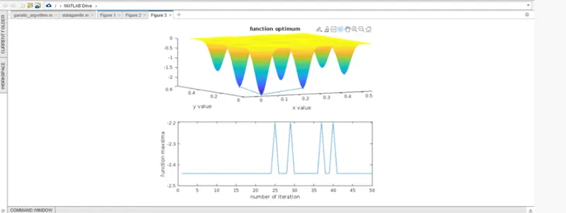
figure(3)
subplot(2,1,1)
hold on
surfc(xx,y,f)
xlabel('x value')
ylabel('y value')
%removing grid line from the surface 
shading interp

plot3(opt_solution_x,opt_solution_y,fval,'Marker','*','MarkerSize',3)
title('function optimum')
subplot(2,1,2)
plot(fval)
xlabel('number of iteration')
ylabel('function maxsima')

Explanation :

first we have to start the program by clear all,close all,clc
then we hav to define the stalagamite function
then we have to write the code for evaluating stalagamite function
then we have to use the ganetic algorithm for eleminating some options
then we have apply this concept for defferent case such as for bounded region ,unbounded region and by increaing the size of the population.

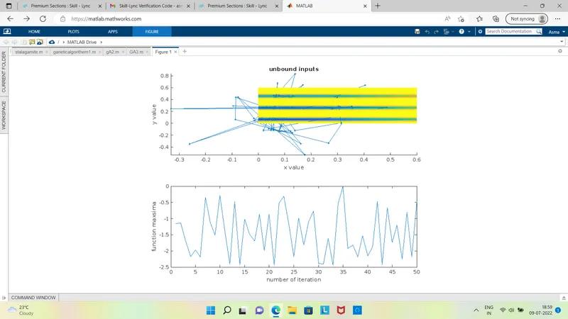
output for case 1:

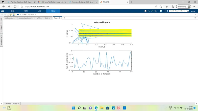
output for case 2:

output for case 3

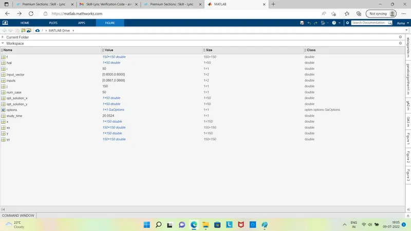
output for work space:

Week 4.1 - Genetic Algorithm

Aim: Is to Try to understand the concept of genetic algorithm by referring to varius sources before you attend this challenge. Look out for information regarding stalagmite function and ways to optimise it.

Genetic algorithms (GA)

Ship work like this
in your own course.

Talk to a career counsellor

Aim: Is to Try to understand the concept of genetic algorithm by referring to varius sources before you attend this challenge. Look out for information regarding stalagmite function and ways to optimise it.

Genetic algorithms (GA)

Ship work like thisin your own course.

Talk to a career counsellor

Ship work like this
in your own course.