Project 2 - Rankine cycle Simulator
Aim:Is to Understand the concept of Rankine cycle by referring to standard thermal engineering text book.
- Create a Rankine Cycle Simulator using OCTAVE/MATLAB.
- Your code should calculate the state points of the Rankine Cycle (any type of your choice) based on user inputs.
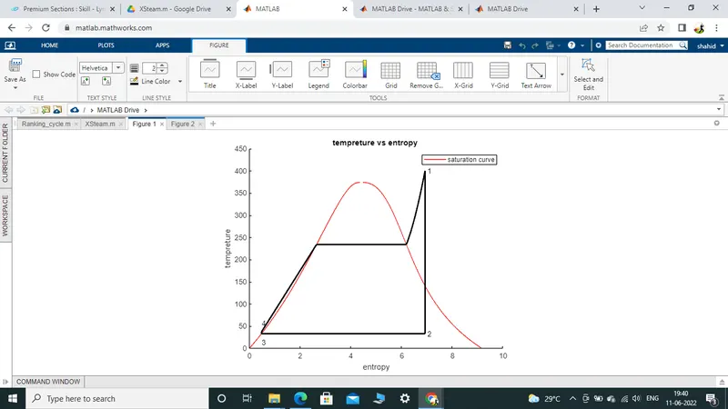
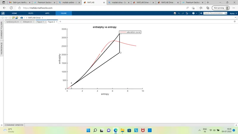
- Then, plot the corresponding T-s and h-s plots for the given set of inputs. Title and axes labels are a must, while legends could be used if necessary.
- The presentation of your code will be taken into consideration while grading. Labelling sections of your code using comments is appreciated.
- Attach a report explaining the working of a rankine cycle simulator and also the research done by you.
Theory:
Rankine cycle
The Rankine cycle is the fundamental operating cycle of all power plants where an operating fluid is continuously evaporated and condensed. The selection of operating fluid depends mainly on the available temperature range. Figure 1 shows the idealized Rankine cycle.
The pressure-enthalpy (p-h) and temperature-entropy (T-s) diagrams of this cycle are given in Figure 2. The Rankine cycle operates in the following steps:
-
1-2-3 Isobaric Heat Transfer. High pressure liquid enters the boiler from the feed pump (1) and is heated to the saturation temperature (2). Further addition of energy causes evaporation of the liquid until it is fully converted to saturated steam (3).
-
3-4 Isentropic Expansion. The vapor is expanded in the turbine, thus producing work which may be converted to electricity. In practice, the expansion is limited by the temperature of the cooling medium and by the erosion of the turbine blades by liquid entrainment in the vapor stream as the process moves further into the two-phase region. Exit vapor qualities should be greater than 90%.
-
4-5 Isobaric Heat Rejection. The vapor-liquid mixture leaving the turbine (4) is condensed at low pressure, usually in a surface condenser using cooling water. In well designed and maintained condensers, the pressure of the vapor is well below atmospheric pressure, approaching the saturation pressure of the operating fluid at the cooling water temperature.
-
5-1 Isentropic Compression. The pressure of the condensate is raised in the feed pump. Because of the low specific volume of liquids, the pump work is relatively small and often neglected in thermodynamic calculations.
Figure 2. T-s and p-h diagrams.
The efficiency of power cycles is defined as
Values of heat and work can be determined by applying the First Law of Thermodynamics to each step. The steam quality x at the turbine outlet is determined from the assumption of isentropic expansion, i.e.,
where is the entropy of vapor and Si* the entropy of liquid
main code for ranking cycle fallows below:
% writting a code to stimulate the Ranking cycle simulter
clear all
close all
clc
% displyaing the ranking cycle and its process
disp('Ranking cycle');
disp('1-2 is isen tropic expanion in turbine ');
disp('2-3 is contant presure heat removal in condensar');
disp('3-4 is isen tropic copmpresion in pump');
disp('4-1 is constant presure heat addition in boiler');

%
%definig the inputs
p1=input('nvalue of presure at turbine inlet ,p1(in bar)= ');
T1=input('nvalue of tempreture at condenser inlet,T1(in C)= ');
p2=input('nvalue of presure at condenser inlet ,p2(in bar)= ');

% taking data from the state 1
h1=XSteam('h_pt',p1,T1);     % enthalphy at state 1
s1=XSteam('s_pt',p1,T1);    %entropy at state 1

% taking data from state 2
s2=s1;
sf2=XSteam('sL_p',p2);     % saturTED liquid entropy
sg2=XSteam('sV_p',p2);      %saturated vapour entropy
x2=(s2-sf2)/(sg2-sf2);
hf2=XSteam('hL_p',p2);
hg2=XSteam('hV_p',p2);
h2=hf2+(x2*(hg2-hf2));


%taking data at state 3
p3=p2;
s3=XSteam('sL_p',p3);
h3=XSteam('hL_P',p3);


%at state 3
s4=s3;
p4=p1;


% work done to run the turbine
wt=h1-h2;


%work doen to run the pump
v3=XSteam('vL_p',p3);
wp=v3*(p4-p3)*100;
h4=h3+wp;


%net work done
Wnet=wt-wp;

%heat input inside the boiler
Qin =h1-h4;

%heat output inside the conenser
Qout=h2-h3;

% calculating the thermal efficiency
eff=(Wnet/Qin)*100;

%specific steam consumpetion  this is nothing but the mass flow rate
%diviede by power
SSC=(3600/Wnet);

%calculating tempreture at state points
T3=XSteam('Tsat_p',p3);
T2=T3;
Cp4=XSteam('Cp_ps',p4,s4);
Cv4=XSteam('Cv_ps',p4,s4);
k=Cp4/Cv4;
T4=T3/((p3/p4)^((k-1)/k));

% calculationg the tempreture entropy enthalpy at vapour state
T6=XSteam('Tsat_p',p1);
s5=XSteam('sL_p',p1);
s6=XSteam('sV_p',p1);
h5=XSteam('hL_P',p1);
h6=XSteam('hV_p',p1);
T5=T6;

%plotting the saturation curve

T=linspace(1,375,1000);
for i=1:length(T)
    sf(i)=XSteam('sL_T',T(i));
    sg(i)=XSteam('sV_T',T(i));
    hf(i)=XSteam('hL_T',T(i));
    hg(i)=XSteam('hV_T',T(i));
end

%plotting the t-s diagram
figure(1)
hold on
plot(sf,T,'r','linewidth',1)
plot(sg,T,'r','linewidth',1)
plot([s1 s2],[T1 T2],'k','linewidth',2)
plot([s2 s3],[T2 T3],'k','linewidth',2)
plot([s3 s4],[T3 T4],'k','linewidth',2)
plot([s4 s5],[T4 T5],'k','linewidth',2)
plot([s5 s6],[T5 T6],'k','linewidth',2)
sc1=linspace(s6, s1, 1000);
for l=1:length(sc1)
    Tc1(l)=XSteam('T_ps',p1,sc1(l));
end
plot(sc1,Tc1,'k','linewidth',2)
text(s1+0.1,T1,'1')
text(s2+0.1,T2,'2')
text(s3,T3-20,'3')
text(s4,T4+20,'4')
title('tempreture vs entropy ')
xlabel('entropy')
ylabel('tempreture')
legend('saturation curve')

%ploting h-s diagram
figure(2)
hold on
plot(sf,hf,'r','linewidth',1)
plot(sg,hg,'r','linewidth',1)
plot([s1 s2],[h1 h2],'k','linewidth',2)
plot([s2 s3],[h2 h3],'k','linewidth',2)
plot([s3 s4],[h3 h4],'k','linewidth',2)
hc=linspace(h4,h5,100);
for k=1:length(hc)
    sch(k)=XSteam('s_ph',p1, hc(k));
end
plot(sch,hc,'k','linewidth',2)
plot([s5 s6],[h5 h6],'k','linewidth',2)
for m=1:length(sc1)
    hc1(m)=XSteam('h_ps',p1,sc1(m));
end

plot(sc1,hc1,'k','linewidth',2)
text(s1+0.1,h1,'1')
text(s2+0.1,h2,'2')
text(s3,h3-100,'3')
text(s4,h4+200,'4')
title('enthalphy vs entropy ')
xlabel('entropy')
ylabel('enthalphy')
legend('saturation curve')


%displing the result
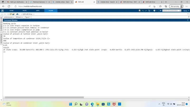
disp('result')
fprintf('at state 1:n');
fprintf('p1:%8.3f barn/n',p1);
fprintf('T1:%8.3f C /n',T1);
fprintf('h1:%8.3f kj/kg /n',h1);
fprintf('s1:%8.3f kj/kgk /n',s1);
fprintf('at state point  2:n');
fprintf('p2:%8.3f barn',p2);
fprintf('T2:%8.3f Cn',T2);
fprintf('h2:%8.3f kj/kgn',h2);
fprintf('s2:%8.3f kj/kgkn',s2);
fprintf('at state point 3:n/n');
fprintf('p3:%8.3f barn',p3);
fprintf('T3:%8.3f Cn',T3);
fprintf('h3:%8.3f kj/kgn',h3);
fprintf('s3:%8.3f kj/kgkn',s3);
fprintf('at state point 4:n/n');
fprintf('p4:%8.3f barn',p4);
fprintf('T4:%8.3f Cn',T4);
fprintf('h4:%8.3f kj/kgn',h4);
fprintf('s4:%8.3f kj/kgkn',s4);
fprintf('turbine work:%8.3f kj/kgn',wt);
fprintf('pump work:%8.3f kj/kgn',wp);
fprintf('Wnet :%8.3f kj/kgn',Wnet);
fprintf('effeciency : %8.3 percent n',eff);
fprintf('ssc: %8.3f kj/kwh',SSC)
Explanetion:
- first we have to start the code by clear all,close all,clc tent we haveto calculate the e
- then we have to extracts the data from the XSteam tabel for enthalphy,entropy and tempretue
- and after that we have to input the value for presure and tempreture as mentioned in th question
- with this quatity and the xsteam table content we have to calculate the entropy anthalphy and tempreture of the rankine cycle
- after that we have to plot the graphs for tempreture vs enthalpy and entropy vs enthalpy
outputs:
1) tempreture vs entropy
2) entropy vs enthalpy
command window output: