Week 4.1 - Genetic Algorithm

AIM:- Write a code in MATLAB to optimize the stalagmite function and find the Global Maxima of the function.

Objective:- 1. Understand the concept of genetic algorithm, and explain the ga syntax.

2. Find the Global maxima for the stalagmite function in MATLAB.

Theory:-

Optimization: It is a decision-making process, which helps us to find the best results. It is a procedure that is executed iterative, by comparing various solutions till an optimum or a satisfactory solution is found.

For Example, in the case of the designing of the simply supported beam to withstand (1-tonne load ), we consider several values like length, breadth, height, the factor of safety, load, and stress. Here optimization helps to find the best values for the length, breadth, height, the factor of safety, load, and stress in such a way that material consumed and stress induced within the limit.

Here are the two techniques available to perform the optimization

1. Deterministic value method- It is the technique where the output of the model is fully determined by the parameters values and initial conditions.
2. Stochastic method -It is like a probabilistic approach.

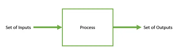
What is GENETIC ALGORITHM:-

1. It is one of the optimization processes.
2. It is a search-Based optimization technique based on the principle of Genetic and Natural selection.
3. It is frequently used to find the optimal and real optimal solutions '
4. It solves the optimization problems in research and machine learning.

Genetic Algorithms are sufficiently randomized in nature, but they perform much better than random local search (in which we just try various random solutions, keeping track of the best so far), as they exploit historical information as well.

The genetic algorithm uses three main types of rules at each step to create the next generation from the current population:

• Selection rules select the individuals, called parents, that contribute to the population of the next generation.
• Crossover rules combine two parents to form children for the next generation.
• Mutation rules apply random changes to individual parents to form children.

How the Genetic Algorithm Works

Outline of the Algorithm

The following outline summarizes how the genetic algorithm works:

• The algorithm begins by creating a random initial population.
• The algorithm then creates a sequence of new populations. At each step, the algorithm uses the individuals in the current generation to create the next population. To create the new population, the algorithm performs the following steps:

1. Scores each member of the current population by computing its fitness value. These values are called the raw fitness scores.
2. Scales the raw fitness scores to convert them into a more usable range of values. These scaled values are called expectation values.
3. Selects members, called parents, based on their expectations.
4. Some of the individuals in the current population that have lower fitness are chosen as elite. These elite individuals are passed on to the next population.
5. Produces children from the parents. Children are produced either by making random changes to a single parent—mutation—or by combining the vector entries of a pair of parents—
6. Replaces the current population with the children to form the next generation.

Syntax for ga- ga(@stalagmite,2,[ ],[ ],[ ],[ ],[0;0],[1;1],[ ],[ ],options)
ga(fun,nvars,A,b,Aeq,beq,lb,ub,nonlcon,options)

ga - Genetic Algorithm
fun - finds a local minimum to function
nvars - number of variables.
A - Linear Inequality Constraints, specified as a real matrix
b - Linear Inequality Constraints, specified as a real vector
Aeq - Linear equality Constraints, specified as a real matrix
beq - Linear equality Constraints, specified as a real matrix
lb - Lower bound
ub- Upper bound
nonlcon - Nonlinear Constraints, specified as a function handle
options- Optimization options, specified as the output

Explanation of writing the MATLAB CODE

1. Staring with clear all, close all, and clc are basic commands used for clearing the memory.
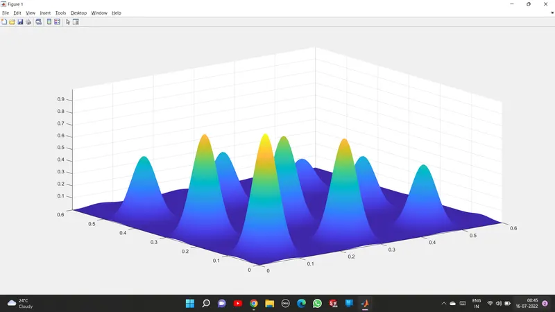
2. After that, I declare the values of x and y with space command in the range between linspace(0,0.6,150)
3. After that, we find out the 2-D array of [xx yy].
4. for finding the global maxima values we use the for loop for recalling the value of x and y 50 times as we declare num_cases=50.
5. Here we use three steps

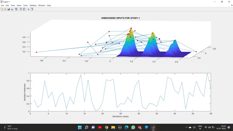
. Giving the input iterations for unbounded region

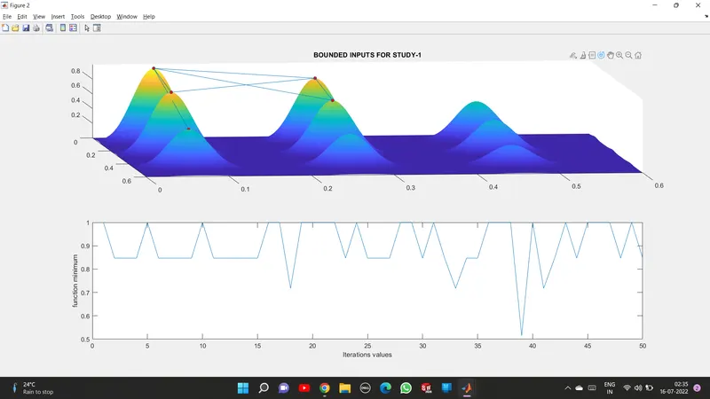
. Giving the iterations for the bounded region in between [0 0], and [1 1]

. Increasing the population size for obtaining the best result and global values

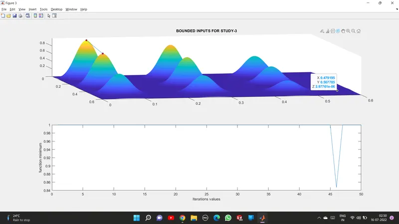
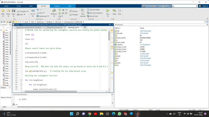
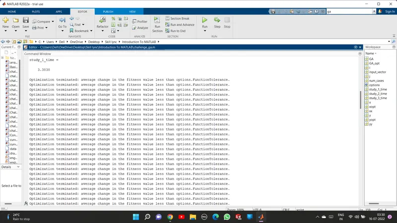
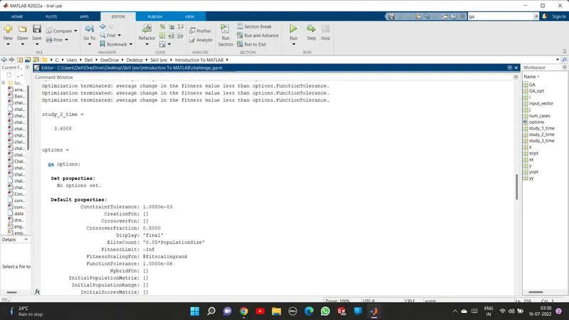
MATLAB CODE

% MATLAB code for optimising the stalagmite function and finding the global maxima of the function

clear all

close all

clc

%Space search inputs are given below

x=linspace(0,0.6,150);

y=linspace(0,0.6,150);

num_cases=50;

%num_cases=50   %GA does not know the values can go beyond or below 0 and 0.6 so we are giving the number of iterations for GA 

[xx yy]=meshgrid(x,y);   % Creating the two dimensional array

%Calling the stalagmite function 

for i=1:length(xx)

    for j=1:length(yy)

        input_vector(1)=xx(i,j);

        input_vector(2)=yy(i,j);

        GA(i,j)=stalagmite_function(input_vector);

    end 
end

%Study-1 Statistical Behaviour for unbounded conditions

tic              %tic-toc commands are used for calculating the iteration time

for i=1:num_cases

    [input_vector,GA_opt(i)]=ga(@stalagmite_function,2);

    xopt(i)=input_vector(1);

    yopt(i)=input_vector(2);

end 

study_1_time=toc

%Plotting the graph for study 1

figure(1)

subplot(2,1,1)

hold on 

surfc(xx,yy,-GA)

shading interp

plot3(xopt,yopt,-GA_opt,'marker','o','MarkerSize',5,'MarkerFaceColor','r')

title('UNBOUNDED INPUTS FOR STUDY-1')

subplot(2,1,2)

plot(-GA_opt)

xlabel('Iterations values')

ylabel('function minimum')

%Study-2 Statistical Behaviour for lower bound and upper bound conditions

tic              %tic-toc commands are used for calculating the iteration time

for i=1:num_cases

    [input_vector,GA_opt(i)]=ga(@stalagmite_function,2,[],[],[],[],[0;0],[1;1]);

    xopt(i)=input_vector(1);

    yopt(i)=input_vector(2);

end 

study_2_time=toc

%Plotting the graph for study 2

figure(2)

subplot(2,1,1)

hold on 

surfc(xx,yy,-GA)

shading interp

plot3(xopt,yopt,-GA_opt,'marker','o','MarkerSize',5,'MarkerFaceColor','r')

title('BOUNDED INPUTS FOR STUDY-2')

subplot(2,1,2)

plot(-GA_opt)

xlabel('Iterations values')

ylabel('function minimum')

%Study-3 Statistical Behaviour for Increasing the GA population

options=optimoptions('ga')   %Calculating the optimum solution for ga and save in options name variabe

options=optimoptions(options,'PopulationSize',240)    %Increasing the population size

tic              %tic-toc commands are used for calculating the iteration time

for i=1:num_cases

    [input_vector,GA_opt(i)]=ga(@stalagmite_function,2,[],[],[],[],[0;0],[1;1],[],[],options);

    xopt(i)=input_vector(1);

    yopt(i)=input_vector(2);

end 

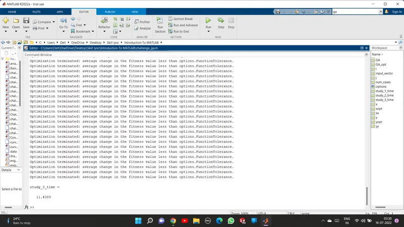
study_3_time=toc

%Plotting the graph for study 3

figure(3)

subplot(2,1,1)

hold on 

surfc(xx,yy,-GA)

shading interp

plot3(xopt,yopt,-GA_opt,'marker','o','MarkerSize',5,'MarkerFaceColor','r')

title('BOUNDED INPUTS FOR STUDY-3')

subplot(2,1,2)

plot(-GA_opt)

xlabel('Iterations values')

ylabel('function minimum')

Result and Conclusion:-

While performing multiple iterations to get the Global maxima in the desired range. For doing is to get the only 1 desired optimum output that is required for a given problem.

Study time will increase by increasing the number of iterations by increasing the Genetic algorithm principle.