Week 3 - Solving second order ODEs

https://youtu.be/kgoSv2lUjuc

Aim: Write a MATLAB code that will simulate the pendulum motion. Simulate the motion between 0-20 sec, for angular displacement=0, angular velocity=3rad/sec at time t=0.

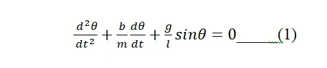
Objective: Our objective is to solve the following ODE. This ODE represents the equation of motion of a simple pendulum with damping.

Theory: In engineering, ODE is used to describe the transient behavior of a system. A simple example is a simple pendulum motion. The way the pendulum moves depends upon Newton's second law. When this law is written down, we get a second-order ordinary differential equation that describes the motion of the “ball” w.r.t. time Let us suppose we have one marker having size (m) is hinged at a fixed point with the help of sting having a length(l). When the ball is displaced at the angle of and then released, the pendulum moves back and forth motion in periodic motion

The equation of the pendulum with damping is given by:

This is a second-order ODE equation, which must be converted into first-order ODE to solve it in the MATLAB with the help of the inbuilt solver Ode45

DERIVATION FOR TO CONVERTING SECOND-ORDER ODE INTO FIRST-ORDER ODE

Let,

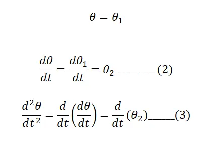
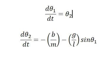
By solving equations (1),(2), and (3), we get the following results

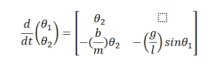
In Matrix form how the theta1 and theta2 will be calculated

The following parameters are assumed to solve this simple pendulum equation

Length (l) = 1 meter

Mass of Bob (m) = 1 kg

Damping coefficient (b) = 0.05

Gravity (g) = 9.81 m/s^2

Time span = 0-20 sec

Angular displacement = 0

Angular velocity = 3 rad/sec

Results and conclusions:

1. Successfully drawn the graph which shows the periodic motion of the simple pendulum

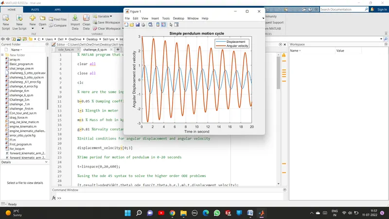
2. From the above experiment, we conclude that the frequency and period of the pendulum are independent of the initial angular displacement amplitude.

% MATLAB program that will simulate the motion of the simple pendulum.

clear all 

close all

clc

% Here are some input parameters that are given to us in the question

b=0.05 % Damping coefficient 

l=1 %length in meter 

m=1 % Mass of bob in kg 

g=9.81 %Grvaity constant in m/s^2

%Initial conditions for angular displacement and angular velocity 

displacement_velocity=[0;3]

% The Time period for the motion of a pendulum in 0-20 seconds

t=linspace(0,20,600);

%using the ode 45 syntaxes to solve the higher-order ODE problems 

[t,result]=ode45(@(t,theta) ode_func(t,theta,b,g,l,m),t,displacement_velocity);


figure(1)

plot(t,result(:,1),'LineWidth',1)

hold on 

plot(t,result(:,2),'LineWidth',2)

title("Simple pendulum motion cycle")

legend("Displacement","Angular velocity")

grid on 

xlabel('Time in second')

ylabel(' Angular Displacement and velocity)

%Pendulum motion simulation

%Input coordinates provided for the initial position of the pendulum 

x0=0;

y0=0;

ct=1;

for i=1:length(t)
    
    theta=result(i,1);
    
    x1=l*sin(theta);
   
    y1=l*(-cos(theta));

figure(2)

plot([-1 1],[0 0],'LineWidth',5,'Color','g')

hold on 

plot([x0 x1],[y0 y1],'LineWidth',2,'Color','r')

hold on 

plot(x0,y0,'Marker','o','MarkerSize',5,'MarkerFaceColor','y')

plot(x1,y1,'Marker','o','MarkerSize',10,'MarkerFaceColor','b')

title('Motion of pendulum')

legend("Supported rod","Length of sting","Fixed point","Bob of Pendulum")

xlabel('X-axis')
ylabel('Y-axis')

hold off

axis([-5 5 -5 5])

grid on 

M(ct)=getframe(gcf)

ct=ct+1;

end 

movie(M)

videofile=VideoWriter('Pendulum motion.avi','Uncompressed AVI')

open(videofile)

writeVideo(videofile,M)

close