Week 4.1 - Genetic Algorithm
%-------------------Challenge Week 4.1- Genetic Algorithm------------------
%--------------To optimize the Stalagmite function using the genetic
%algorithm technique to find the global maxima-----------------------------

clear
close
clc


%Defining searchspace x and y
x = linspace(0,0.6,150);
y = linspace(0,0.6,150);

%Creating 2-D for the searchspace
[xx, yy] = meshgrid(x,y);

%Working out the Stalagmite function
for i=1:length(xx)
    for j=1:length(yy)
        input_vect(1) = xx(i,j);
        input_vect(2) = yy(i,j);
        f(i,j) = stalagmite(input_vect);
    end
end
figure(1)
surf(xx, yy, -f)
shading interp
xlabel('x axis')
ylabel('y axis')
zlabel('stalagmite f')
title('Stalagmite Function')

%Running the ga for various cases for 50 times
num_cases = 50;
tic
%----Case 1 unbounded study
for i = 1 : num_cases
    [inputs, fopt(i)] = ga(@stalagmite,2);
    xopt(i) = inputs(1);
    yopt(i) = inputs(2);
end

case1_time = toc

figure(2)
subplot(2,1,1)
hold on
surfc(xx,yy,-f)
shading interp
plot3(xopt,yopt,-fopt,Marker="o",MarkerSize=5,MarkerFaceColor="r")
xlabel('x axis')
ylabel('y axis')
zlabel('stalagmite f')
legend('Stalagmite Surface','Stalagmite Contour','GA Results')
title('Unbounded Study')
subplot(2,1,2)
plot(-fopt)
xlabel('iterations')
ylabel('function maxima')


tic
%----Case 2 bounded study
for j = 1 : num_cases
    [inputs, fopt(j)] = ga(@stalagmite,2,[],[],[],[],[0;0],[0.4;0.4]);
    xopt(j) = inputs(1);
    yopt(j) = inputs(2);
end

case2_time = toc

figure(3)
subplot(2,1,1)
hold on
surfc(xx,yy,-f)
shading interp
plot3(xopt,yopt,-fopt,Marker="o",MarkerSize=5,MarkerFaceColor="r")
xlabel('x axis')
ylabel('y axis')
zlabel('stalagmite f')
legend('Stalagmite Surface','Stalagmite Contour','GA Results')
title('Bounded Study')
subplot(2,1,2)
plot(-fopt)
xlabel('iterations')
ylabel('function maxima')

tic
%----Case 3 bounded study with Population size
options = optimoptions('ga');
options = optimoptions(options,"PopulationSize",270);
for k = 1 : num_cases
    [inputs, fopt(k)] = ga(@stalagmite,2,[],[],[],[],[0;0],[0.4;0.4],[],[],options);
    xopt(k) = inputs(1);
    yopt(k) = inputs(2);
end

case3_time = toc

figure(4)
subplot(2,1,1)
hold on
surfc(xx,yy,-f)
shading interp
plot3(xopt,yopt,-fopt,Marker="o",MarkerSize=5,MarkerFaceColor="r")
xlabel('x axis')
ylabel('y axis')
zlabel('stalagmite f')
legend('Stalagmite Surface','Stalagmite Contour','GA Results')
title('Bounded Study With Population Size')
subplot(2,1,2)
plot(-fopt)
xlabel('iterations')
ylabel('function maxima')


----------------------------------------------------------------------------------------
%----------------Stalagmite Function----------------------------------------------------

function [f] = stalagmite(input_vector)
x = input_vector(1);
y = input_vector(2);

f1_x = (sin((5.1*pi*x)+0.5))^6;
f1_y = (sin((5.1*pi*y)+0.5))^6;

tr_1 = ((x-0.0667)^2)/0.64;
f2_x = exp(-4*log(2)*tr_1);

tr_2 = ((y-0.0667)^2)/0.64;
f2_y = exp(-4*log(2)*tr_2);

f = - ((f1_x)*(f2_x)*(f1_y)*(f2_y));
end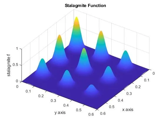
Aim:
Write a program to find the global maxima of the stalagmite function using genetic algorithm.
Equations Used:
Stalagmite Function:
`f_1x= [sin〖5.1πx+0.5〗]^6`
`f_1y= [sin〖5.1πy+0.5〗]^6`
`f_2x=exp[-4 ln2 (x-0.0667)^2/0.64]`
`f_2y=exp[-4 ln2 (y-0.0667)^2/0.64]`
`f_(x,y)= f_1x f_2x f_1y f_2y`
Theory:
Genetic Algorithm
In computer science and operations research, a genetic algorithm (GA) is a metaheuristic inspired by the process of natural selection that belongs to the larger class of evolutionary algorithms (EA). Genetic algorithms are commonly used to generate high-quality solutions to optimization and search problems by relying on biologically inspired operators such as mutation, crossover and selection. In a genetic algorithm, a population of candidate solutions (called individuals, creatures, organisms, or phenotypes) to an optimization problem is evolved toward better solutions. Each candidate solution has a set of properties (its chromosomes or genotype) which can be mutated and altered.
The evolution usually starts from a population of randomly generated individuals, and is an iterative process, with the population in each iteration called a generation. In each generation, the fitness of every individual in the population is evaluated; the fitness is usually the value of the objective function in the optimization problem being solved. The more fit individuals are stochastically selected from the current population, and each individual's genome is modified (recombined and possibly randomly mutated) to form a new generation. The new generation of candidate solutions is then used in the next iteration of the algorithm. Commonly, the algorithm terminates when either a maximum number of generations has been produced, or a satisfactory fitness level has been reached for the population.
A typical genetic algorithm requires:
- a genetic representation of the solution domain,
- a fitness function to evaluate the solution domain.
Once the genetic representation and the fitness function are defined, a GA proceeds to initialize a population of solutions and then to improve it through repetitive application of the mutation, crossover, inversion and selection operators.
Initialization
The population size depends on the nature of the problem, but typically contains several hundreds or thousands of possible solutions. Often, the initial population is generated randomly, allowing the entire range of possible solutions (the search space). Occasionally, the solutions may be "seeded" in areas where optimal solutions are likely to be found.
Selection
During each successive generation, a portion of the existing population is selected to breed a new generation. Individual solutions are selected through a fitness-based process, where fitter solutions (as measured by a fitness function) are typically more likely to be selected. Certain selection methods rate the fitness of each solution and preferentially select the best solutions. Other methods rate only a random sample of the population, as the former process may be very time-consuming.
The fitness function is defined over the genetic representation and measures the quality of the represented solution. The fitness function is always problem dependent.
Genetic operators
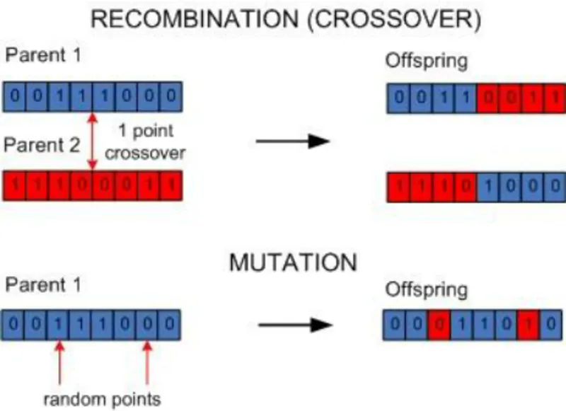
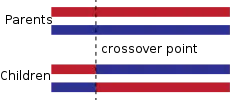
The next step is to generate a second generation population of solutions from those selected, through a combination of of genetic operators: crossover (also called recombination), and mutation.
For each new solution to be produced, a pair of "parent" solutions is selected for breeding from the pool selected previously. By producing a "child" solution using the above methods of crossover and mutation, a new solution is created which typically shares many of the characteristics of its "parents". New parents are selected for each new child, and the process continues until a new population of solutions of appropriate size is generated.
Termination
This generational process is repeated until a termination condition has been reached. Common terminating conditions are:
- A solution is found that satisfies minimum criteria
- Fixed number of generations reached
- Allocated budget (computation time/money) reached
- The highest ranking solution's fitness is reaching or has reached a plateau such that successive iterations no longer produce better results
- Manual inspection
- Combinations of the above
Genetic Algorithm in MATLAB:
- MATLAB has the solver for genetic algorithm named ‘ga’ in-built in the optimization toolbox.
- By default, the ‘ga’ in MATLAB optimizes the given function for the minimum.
- The syntax of ga is given by
[x,fval] = ga(fun,nvars,A,b,Aeq,beq,lb,ub,nonlocn,intcon,options)
- x – vector containing the values where the function is minimum
- fval – the fitness value of the function
- fun – the function that needs to be optimized
- A,b – linear inequalities, specify [ ] if not applicable
- Aeaq, beq – linear equalities, specify [ ] if not applicable
- lb, ub – lower and upper bounds to instruct the ga to set the search space
- nonlcon – Nonlinear constraints, specified as a function handle or function name. nonlcon is a function that accepts a vector or array x and returns two arrays, c(x) and ceq(x). Specify [ ] if not applicable.
- intcon – Indices of integer variable. Specify [ ] if not applicable.
- options – other optimization options created using ‘optimoptions’
Explanation:
Stage 1:
%-------------------Challenge Week 4.1- Genetic Algorithm------------------
%--------------To optimize the Stalagmite function using the genetic
%algorithm technique to find the global maxima-----------------------------
clear
close
clc
%Defining searchspace x and y
x = linspace(0,0.6,150);
y = linspace(0,0.6,150);
%Creating 2-D for the searchspace
[xx, yy] = meshgrid(x,y);
%Working out the Stalagmite function
for i=1:length(xx)
for j=1:length(yy)
input_vect(1) = xx(i,j);
input_vect(2) = yy(i,j);
f(i,j) = stalagmite(input_vect);
end
end
figure(1)
surf(xx, yy,f)
shading interp
xlabel('x axis')
ylabel('y axis')
zlabel('stalagmite f')
title('Stalagmite Function')
- First step is to define the function space in x and y axes ‘linspace’ command is used to generate the space as a 1-D array.
- Since the stalagmite function requires two dimensional attributes the values of the function space are transformed into a 2-D array using the ‘meshgrid’ command.
- With the 2-D data of x and y from the meshgrid are iterated through the last index/position, and for each x and y the stalagmite function is evaluated.
- Then the values of the stalagmite function is plotted in figure, since it is 3 dimensional function ‘surf’ command is used to plot it as a surface and ‘shading interp’ command is used to remove the grid lines and smooth the surface.
- The figure is annotated with axes and title.
Stage 2:
%Running the ga for various cases for 50 times
num_cases = 50;
tic
%----Case 1 unbounded study
for i = 1 : num_cases
[inputs, fopt(i)] = ga(@stalagmite,2);
xopt(i) = inputs(1);
yopt(i) = inputs(2);
end
case1_time = toc
figure(2)
subplot(2,1,1)
hold on
surfc(xx,yy,-f)
shading interp
plot3(xopt,yopt,-fopt,Marker="o",MarkerSize=5,MarkerFaceColor="r")
xlabel('x axis')
ylabel('y axis')
zlabel('stalagmite f')
legend('Stalagmite Surface','Stalagmite Contour','GA Results')
title('Unbounded Study')
subplot(2,1,2)
plot(fopt)
xlabel('iterations')
ylabel('function maxima')
- Next is to perform the optimization using the ‘genetic algorithm’ technique.
- The MATLAB’s in-built solver ‘ga’ is called and is runned for 50 times.
- The case is unbounded, means the ‘ga’ will solve only for the minimum(maximum) value and its x, y values.
- The search space for ‘ga’ will be taken at random at each time of the iteration.
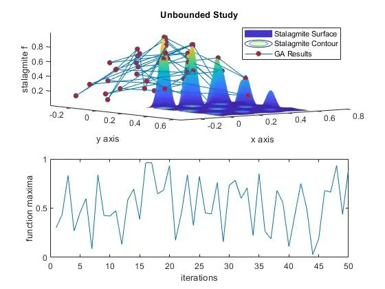
- Then the stalagmite and ga data are plotted using ‘surfc’, ‘subplot’, ’plot3’ and ‘hold on’ commands. The ‘surfc’ plot command will plot the surface and the contour of the attributes. The ‘plot3’ command will plot points and lines in 3 axes system.
- Markers are used to indicate the points clearly and distinctly.
- The plot is annotated with axis labels, title and legend.
- From the plot it can be concluded that the data of ‘ga’ is scattered beyond the stalagmite surface.
- In the beginning and end of the ‘ga’ calculation ‘tic’ and ‘tok’ commands are used to access the stopwatch to note down the time taken to solve for 50 times and is found out to be case1_time = 2.2723 seconds.
Stage 3:
tic
%----Case 2 bounded study
for j = 1 : num_cases
[inputs, fopt(j)] = ga(@stalagmite,2,[],[],[],[],[0;0],[0.4;0.4]);
xopt(j) = inputs(1);
yopt(j) = inputs(2);
end
case2_time = toc
figure(3)
subplot(2,1,1)
hold on
surfc(xx,yy,-f)
shading interp
plot3(xopt,yopt,-fopt,Marker="o",MarkerSize=5,MarkerFaceColor="r")
xlabel('x axis')
ylabel('y axis')
zlabel('stalagmite f')
legend('Stalagmite Surface','Stalagmite Contour','GA Results')
title('Bounded Study')
subplot(2,1,2)
plot(fopt)
xlabel('iterations')
ylabel('function maxima')
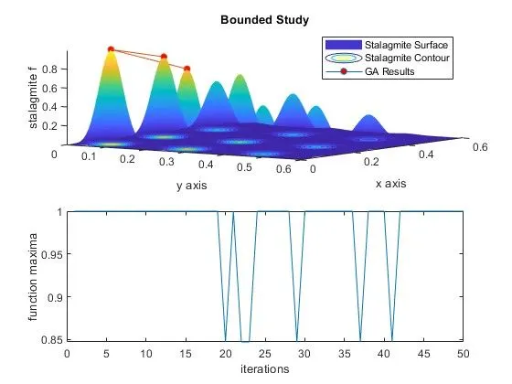
- The ‘ga’ is repeated again for 50 times, but with a distinct boundary in x and y.
- This boundary defines the search space for the ‘ga’.
- Then the stalagmite and ga data are plotted using ‘surfc’, ‘subplot’, ’plot3’ and ‘hold on’ commands. The ‘surfc’ plot command will plot the surface and the contour of the attributes. The ‘plot3’ command will plot points and lines in 3 axes system.
- Markers are used to indicate the points clearly and distinctly.
- The plot is annotated with axis labels, title and legend.
- From the plot it can be concluded that the data of ‘ga’ is within the stalagmite surface and the three most higher peaks there.
- In the beginning and end of the ‘ga’ calculation ‘tic’ and ‘tok’ commands are used to access the stopwatch to note down the time taken to solve for 50 times and is found out to be case2_time = 4.2742 seconds.
Stage 4:
tic
%----Case 3 bounded study with Population size
options = optimoptions('ga');
options = optimoptions(options,"PopulationSize",270);
for k = 1 : num_cases
[inputs, fopt(k)] = ga(@stalagmite,2,[],[],[],[],[0;0],[0.4;0.4],[],[],options);
xopt(k) = inputs(1);
yopt(k) = inputs(2);
end
case3_time = toc
figure(4)
subplot(2,1,1)
hold on
surfc(xx,yy,-f)
shading interp
plot3(xopt,yopt,-fopt,Marker="o",MarkerSize=5,MarkerFaceColor="r")
xlabel('x axis')
ylabel('y axis')
zlabel('stalagmite f')
legend('Stalagmite Surface','Stalagmite Contour','GA Results')
title('Bounded Study With Population Size')
subplot(2,1,2)
plot(fopt)
xlabel('iterations')
ylabel('function maxima')
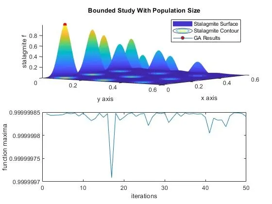
- The ‘ga’ is repeated for the third time for 50 times, with a distinct boundary in x and y and initial population size.
- This boundary defines the search space for the ‘ga’.
- ‘ga’ by default take 50 population data.
- The default solver options can be modified by loading the options using ‘options’ and ‘optimoptions’ command and keyword.
- The population size here is increased to 270.
- Then the stalagmite and ga data are plotted using ‘surfc’, ‘subplot’, ’plot3’ and ‘hold on’ commands. The ‘surfc’ plot command will plot the surface and the contour of the attributes. The ‘plot3’ command will plot points and lines in 3 axes system.
- Markers are used to indicate the points clearly and distinctly.
- The plot is annotated with axis labels, title and legend.
- From the plot it can be concluded that the data of ‘ga’ is within the stalagmite surface and at the highest peak in it.
- In the beginning and end of the ‘ga’ calculation ‘tic’ and ‘tok’ commands are used to access the stopwatch to note down the time taken to solve for 50 times and is found out to be case3_time = 11.6104 seconds.
Stalagmite function – supplementary:
function [f] = stalagmite(input_vector)
x = input_vector(1);
y = input_vector(2);
f1_x = (sin((5.1*pi*x)+0.5))^6;
f1_y = (sin((5.1*pi*y)+0.5))^6;
tr_1 = ((x-0.0667)^2)/0.64;
f2_x = exp(-4*log(2)*tr_1);
tr_2 = ((y-0.0667)^2)/0.64;
f2_y = exp(-4*log(2)*tr_2);
f = - ((f1_x)*(f2_x)*(f1_y)*(f2_y));
end
- Basically, and by default the ‘ga’ solves and finds out the minima of a function.
- Here the ‘stalagmite function’ is used which is also called ‘test function’ by definition means it is a function that is used to test the ‘ga’ if works correct or not.
- The stalagmite function that accepts two inputs and produces an output depending to the inputs.
- The stalagmite function is given by,
`f_(x,y)= f_1x f_2x f_1y f_2y`
`f_1x= [sin〖5.1πx+0.5〗]^6`
`f_1y= [sin〖5.1πy+0.5〗]^6`
`f_2x=exp[-4 ln2 (x-0.0667)^2/0.64]`
`f_2y=exp[-4 ln2 (y-0.0667)^2/0.64]`
- In the coded function the final fx,y is –(ve) signed because the aim is to find the maxima of the function.
Stopping/Termination Criteria:
MATLAB will terminate the ‘ga’ optimization when one or more of the following conditions are met.
- MaxGenerations — Specifies the maximum number of iterations for the genetic algorithm to perform.
- FitnessLimit — The algorithm stops if the best fitness value is less than or equal to the value of FitnessLimit.
- MaxStallGenerations— The algorithm stops if the average relative change in the best fitness function value over MaxStallGenerations is less than or equal to
- MaxStallTime— The algorithm stops if there is no improvement in the best fitness value for an interval of time in seconds specified by
- FunctionTolerance— The algorithm stops if the average relative change in the best fitness function value over MaxStallGenerations is less than or equal to FunctionTolerance.
- ConstraintTolerance — The ConstraintTolerance is not used as stopping criterion. It is used to determine the feasibility with respect to nonlinear constraints. Also, max(sqrt(eps),ConstraintTolerance) determines feasibility with respect to linear constraints.
Errors:
There were no significant errors while execution and coding.
References: