Project 2 - Rankine cycle Simulator

%----------------- Project-2 Rankine Cycle --------------------------------
%------To calculate state points and plot t-s , h-s diagram for rankine
%cycle with user given input-----------------------------------------------

clear all
close all
clc

%Rankine Cycle process flow and naming conventions for program

%Process 1-2 Adiabatic Expansion in the Turbine
%Process 2-3 Isothermal Compression / Condensation at constant pressure
%Process 3-4 Warming/Heating at constant volume
%Process 4-1 Isothermal Expansion at constant pressure

%State Points
% 1- Turbine inlet/Boiler outlet, 2- Condenser inlet/Turbine outlet
% 3- Pump inlet/Condenser outlet, 4- Boiler inlet/Pump outlet

%State Variables
%p1 = Turbine inlet / Boiler outlet Pressure (Bar)
%T1 = Turbine inlet / Boiler outlet Temperature (deg C)
%p2 = Turbine outlet / Condenser inlet Pressure (Bar)

%Display the Rankine Cycle
disp('----------------------------------RANKINE CYCLE----------------------------------------')
disp('Process 1-2 Revesible-Adiabatic/Isentropic Expansion in the Turbine, Work_out')
disp('Process 2-3 Isothermal Heat Rejection at constant pressure in the Condenser, Heat_out')
disp('Process 3-4 Constant volume Compression in the Pump, Work_in')
disp('Process 4-1 Isothermal Heat Addition in Boiler, Heat_in')

%Input Parameters by user
p1 = input('Enter Turbine inlet Pressure (Bar)  : ');
T1 = input('Enter Turbine inlet Temperature (C) : ');
p2 = input('Enter Turbine outlet Pressure (Bar) : ');





%State Variable at State 1 Turbine inlet/Boiler outlet

%Having Pressure and Temperature at Point 1 , Enthalpy, Specific Entropy and Specific Volume
%can be calculated with the help of given XSteam library function file-----

% h1 - Enthalpy in kJ/kg
h1 = XSteam('h_pT',p1,T1);

% s1 - Specific Entropy in kJ/K.kg
s1 = XSteam('s_pT',p1,T1);

% v1 - Specific Volume in m3/kg
v1 = XSteam('v_pT',p1,T1);





%State Variables at State 2 Turbine outlet/Condenser inlet

disp('Since the process 1-2 is adiabatic, s1 = s2.')
disp('Inside the turbine the saturated dry steam falls to lower dryness/vapour fraction.')

s2 = s1;
disp('p2 is an input')

%With the help of of XSteam function
%h2 - Enthalpy in kJ/kg
h2 = XSteam('h_px',p2,XSteam('x_ps',p2,s2));

%T2 - Temperature in C
T2 = XSteam('T_ps',p2,s2);

%v2 - Specific Volume in m3/kg
v2 = XSteam('v_ps',p2,s2);





%State Variables at State 3 Condenser outlet/Pump inlet

disp('Since condensation occurs at constant pressure, p2 = p3.')
p3 = p2;

disp('Vapour/Steam becomes liquid/water in the condenser, Latent heat is removed.')

%With the help of XSteam

%h3 - Enthalpy in kJ/kg
h3 = XSteam('hL_p',p3);

%T3 - Temperature in C
T3 = XSteam('Tsat_p',p3);

%s3 - Specific Entropy in kJ/K.kg
s3 = XSteam('sL_p',p3);

%v3 - Specific Volume in m3/kg
v3 = XSteam('vL_p',p3);





%State Variables at State 4 Pump outlet/Boiler inlet

disp('Water is pumped to the boiler isoentropically, s4 = s3')
s4 = s3;

disp("According to the cycle's theory the pressure is constant on process 4-1")

p4 = p1;

%With the help of XSteam

%h4 - Enthalpy in kJ/kg
h4 = XSteam('h_ps',p4,s4);

%T4 - Temperature in C
T4 = XSteam('T_ps',p4,s4);

%v4 - Specific Volume in m3/kg
v4 = XSteam('v_ps',p4,s4);

%Tracing the change in Entropy and Enthalpy
T_range = linspace(T4,T1,500);
for i = 1:length(T_range)
    %Constant pressure heat addition
    s_range(i) = XSteam('s_pT',p1,T_range(i));
    %Enthalpy change from 2 to 3
    h_range2_3(i) = XSteam('h_ps',p2,s_range(i));
    %Enthalpy change from 4 to 1
    h_range4_1(i) = XSteam('h_ps',p1,s_range(i));
end

disp("----------------------------Plotting in Progress-------------------------------------")

%Plotting process Graphs
%T-s Diagram
figure(1)
hold on
plot([s1 s2],[T1 T2],LineWidth=4,Color='b')
plot([s2 s3],[T2 T3],LineWidth=4,Color='black')
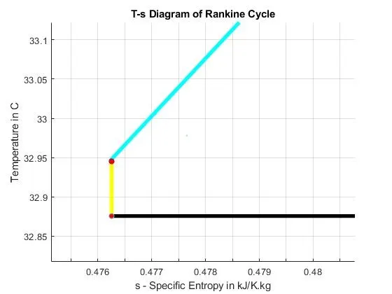
plot([s3 s4],[T3 T4],LineWidth=4,Color='yellow')
plot(s_range,T_range,LineWidth=4,Color='c')
xlabel('s - Specific Entropy in kJ/K.kg')
ylabel('Temperature in C')
legend('Isentropic Expansion','Heat Rejection','Isentropic Compression','Heat Addition',Location='eastoutside')

%h-s Diagram
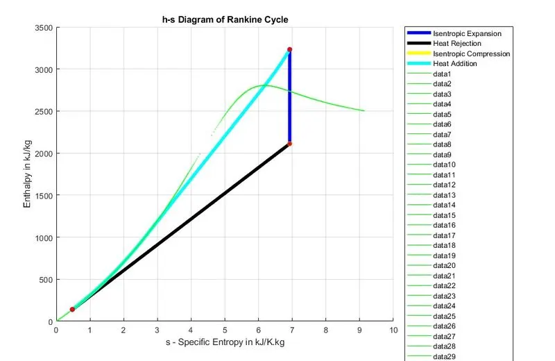
figure(2)
hold on
plot([s1 s2],[h1 h2],LineWidth=4,Color='b')
plot(s_range,h_range2_3,LineWidth=4,Color='black')
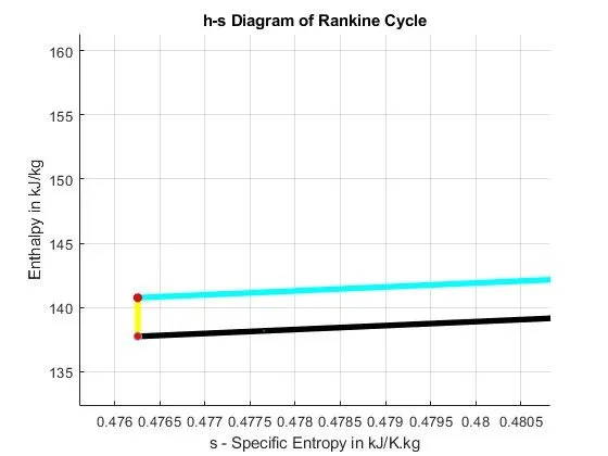
plot([s3 s4],[h3 h4],LineWidth=4,Color='yellow')
plot(s_range,h_range4_1,LineWidth=4,Color='c')
xlabel('s - Specific Entropy in kJ/K.kg')
ylabel('Enthalpy in kJ/kg')
legend('Isentropic Expansion','Heat Rejection','Isentropic Compression','Heat Addition',Location='eastoutside')

%Plotting Critical curve points of water/steam
t_r = linspace(0,374,500);
%T-s
figure(1)
hold on
for j = 1:length(t_r)
    plot(XSteam('sL_T',t_r(j)),t_r(j),Marker=".",MarkerSize=1.5,Color='g')
    plot(XSteam('sV_T',t_r(j)),t_r(j),Marker=".",MarkerSize=1.5,Color='g')
end

%h-s
figure(2)
for j = 1:length(t_r)
    plot(XSteam('sL_T',t_r(j)),XSteam('hL_T',t_r(j)),Marker=".",MarkerSize=1.5,Color='g')
    plot(XSteam('sV_T',t_r(j)),XSteam('hV_T',t_r(j)),Marker=".",MarkerSize=1.5,Color='g')
end

%Plotting State Points
%T-s
figure(1)
hold on
plot(s1,T1,Marker="o",MarkerFaceColor='r',MarkerSize=5.5)
plot(s2,T2,Marker="o",MarkerFaceColor='r',MarkerSize=5.5)
plot(s3,T3,Marker="o",MarkerFaceColor='r',MarkerSize=5.5)
plot(s4,T4,Marker="o",MarkerFaceColor='r',MarkerSize=5.5)
grid on
title('T-s Diagram of Rankine Cycle')

%h-s
figure(2)
hold on
plot(s1,h1,Marker="o",MarkerFaceColor='r',MarkerSize=5.5)
plot(s2,h2,Marker="o",MarkerFaceColor='r',MarkerSize=5.5)
plot(s3,h3,Marker="o",MarkerFaceColor='r',MarkerSize=5.5)
plot(s4,h4,Marker="o",MarkerFaceColor='r',MarkerSize=5.5)
grid on
title('h-s Diagram of Rankine Cycle')


%Calculation
%1 net work output
%Turbine and pump work
Work_tur = h1-h2;
Work_pump = h4-h3;
%Boiler and condenser heat
Q_out_cond = h2-h3;
Q_in_boil = h1-h4;
%Net Work Done
Work_net = Work_tur - Work_pump;
%Back Work Ratio
back_work_ratio = Work_pump/Work_tur;
%Efficiency
effi_rank = (Work_net/Q_in_boil)*100;
%Specific Steam Consumption
SS_C = 1/Work_net;

disp('----------------------------------RESULTS-----------------------------------------')
%States 1,2,3,4

disp("--------------------State Variables at State 1---------------------------------")
disp("Turbine inlet/Boiler outlet, Pressure         p1 = " +p1 +" bar ")
disp("Turbine inlet/Boiler outlet, Temperature      T1 = " +T1 +" C ")
disp("Turbine inlet/Boiler outlet, Enthalpy         h1 = " +h1 +" kJ/kg ")
disp("Turbine inlet/Boiler outlet, Specific Entropy s1 = " +s1 +" kJ/K.kg ")
disp("Turbine inlet/Boiler outlet, Specific Volume  v1 = " +v1 +" m3/kg")

disp(" ")
disp(" ")

disp("--------------------State Variables at State 2---------------------------------")
disp("Condenser inlet/Turbine Outlet, Pressure         p2 = " +p2 +" bar ")
disp("Condenser inlet/Turbine Outlet, Temperature      T2 = " +T2 +" C ")
disp("Condenser inlet/Turbine Outlet, Enthalpy         h2 = " +h2 +" kJ/kg ")
disp("Condenser inlet/Turbine Outlet, Specific Entropy s2 = " +s2 +" kJ/K.kg ")
disp("Condenser inlet/Turbine Outlet, Specific Volume  v2 = " +v2 +" m3/kg")

disp(" ")
disp(" ")

disp("--------------------State Variables at State 3---------------------------------")
disp("Pump inlet/Condenser Outlet, Pressure         p3 = " +p3 +" bar ")
disp("Pump inlet/Condenser Outlet, Temperature      T3 = " +T3 +" C ")
disp("Pump inlet/Condenser Outlet, Enthalpy         h3 = " +h3 +" kJ/kg ")
disp("Pump inlet/Condenser Outlet, Specific Entropy s3 = " +s3 +" kJ/K.kg ")
disp("Pump inlet/Condenser Outlet, Specific Volume  v3 = " +v3 +" m3/kg")

disp(" ")
disp(" ")

disp("--------------------State Variables at State 4---------------------------------")
disp("Boiler inlet/Pump Outlet, Pressure         p4 = " +p4 +" bar ")
disp("Boiler inlet/Pump Outlet, Temperature      T4 = " +T4 +" C ")
disp("Boiler inlet/Pump Outlet, Enthalpy         h4 = " +h4 +" kJ/kg ")
disp("Boiler inlet/Pump Outlet, Specific Entropy s4 = " +s4 +" kJ/K.kg ")
disp("Boiler inlet/Pump Outlet, Specific Volume  v4 = " +v4 +" m3/kg")
disp(" ")
disp(" ")
disp(" ")
disp("Turbine Work,                 Wtur = " +Work_tur +" kJ/kg")
disp("Pump Work,                   Wpump = " +Work_pump +" kJ/kg")
disp("Work Done,                    Wnet = " +Work_net +" kJ/kg ")
disp("Back Work Ratio,               BWR = " +back_work_ratio)
disp("Specific Steam Comsumption,    SSC = " +SS_C+" kg/kJ")
disp("Efficiency,                 N_Rank = " +effi_rank+" %")
disp("-----------------------------EOR--------------------------------------------------")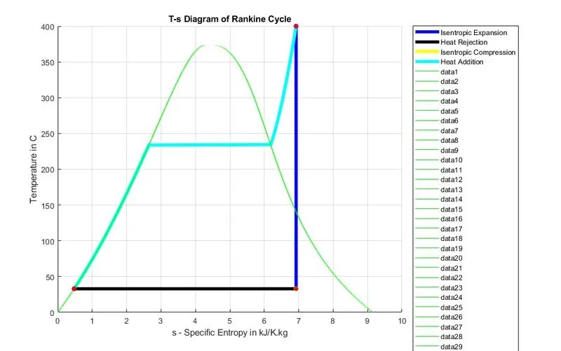

Aim:

To calculate the state points of Rankine Cycle with user inputs and to plot T-s and h-s for the cycle.

Theory:

Rankine Cycle is a thermodynamic vapour cycle which uses water/steam as working substance. It is widely used in steam turbines of power plants.

The cycle consists four processes:

1. Isothermal Expansion
2. Adiabatic Expansion
3. Isothermal Compression
4. Warming/Heating Operation

`W = H_1- H_3`

`η= (H_1- H_3)/(H_1- h_2 )`

1. Isothermal Expansion

The water is isothermally converted into dry saturated steam at constant temperature and pressure. The heat absorbed during this process is the latent heat. H₁=L.

2. Adiabatic Expansion

The dry saturated steam expands adiabatically and there is no change in entropy. The steam falls in pressure and temperature respectively and also dips in dryness fraction.

3. Isothermal Compression

The unsaturated wet steam is now isothermally compressed at constant temperature and pressure until the whole steam is converted/condensed into water. The heat rejected in this process is the latent heat.

4. Warming/Heating Operation

The water is heated/warmed at constant volume. The heat absorbed by the water is equal to the sensible heat.

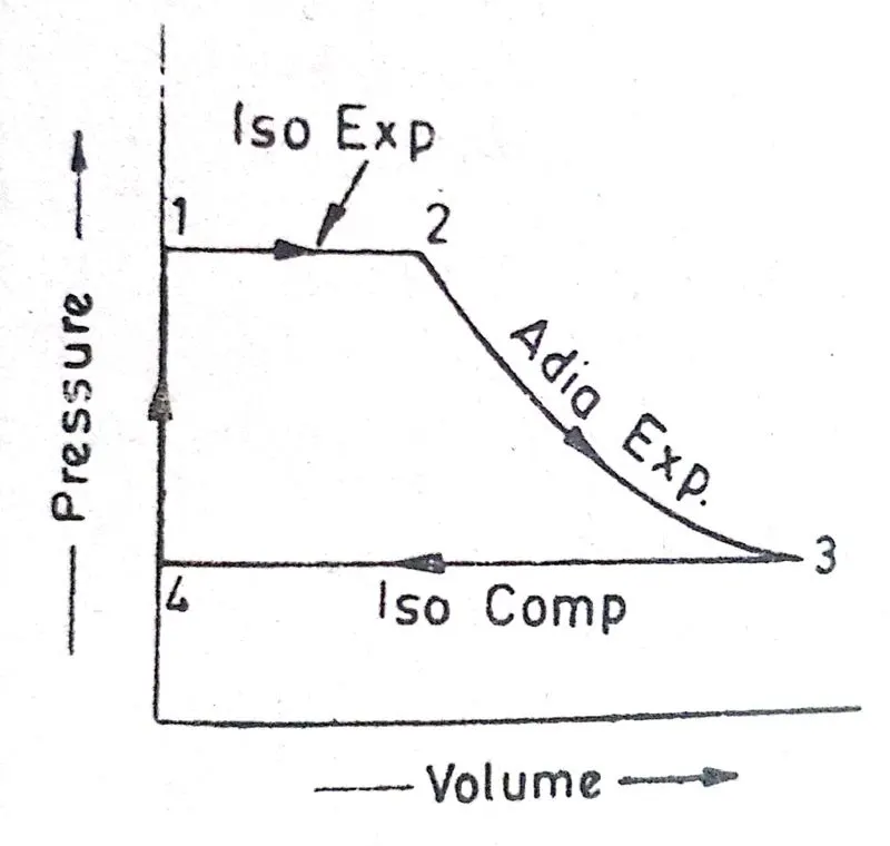
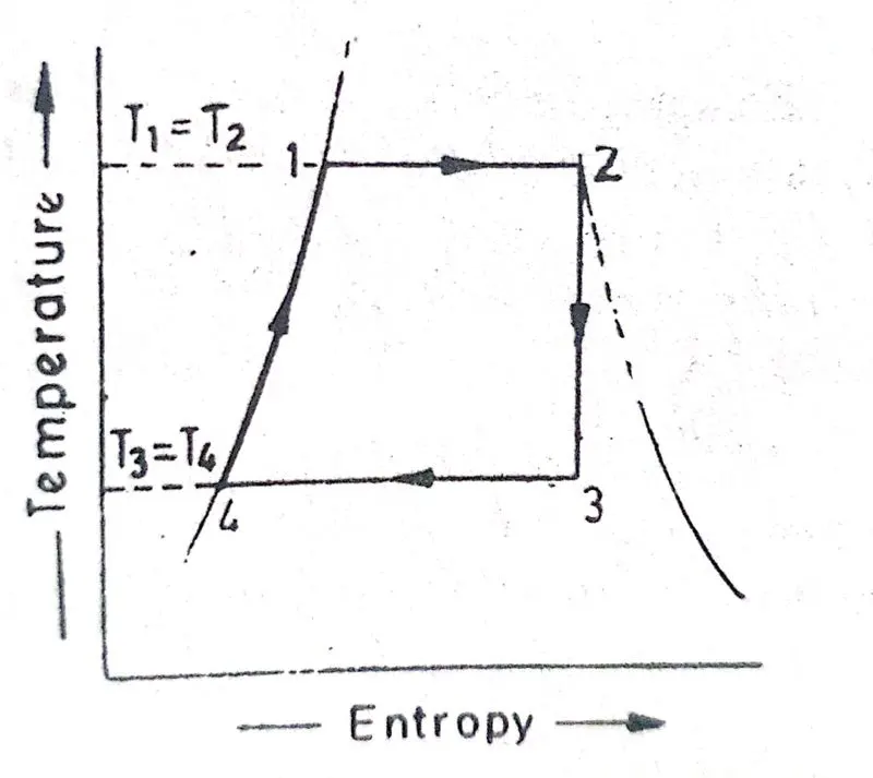
Where,

H – Heat transfer

L – Latent Heat

𝑥 – dryness fraction

h – enthalpy

There are many modified rankine cycles with respect to the desired efficiency.

Equations Used:

Turbine Work Output in kJ/kg:

`W_(tur)= h_1- h_2`

Pump Work Input in kJ/kg:

`W_(pump)= h_4- h_3`

Heat Rejected in Condenser in kJ/kg:

`Q_(out)= h_2- h_3`

Heat Absorbed in Boiler in kJ/kg:

`Q_(IN)= h_1- h_4`

Net Work Done in kJ/kg:

`W_(NET)= W_(tur)- W_(pump)`

Back work ratio :

`BWR= (W_(pump))/(W_(tur))`

Specific Steam Consumption in kg/kJ:

`SSC= 1/W_(NET)`

Efficiency of Rankine cycle :

`η_(rank)= (W_(NET))/(Q_(IN)) ×100`

Explanation:

Stage 1:

%----------------- Project-2 Rankine Cycle --------------------------------

%------To calculate state points and plot t-s , h-s diagram for rankine

%cycle with user given input-----------------------------------------------

clear all

close all

clc

%Rankine Cycle process flow and naming conventions for program

%Process 1-2 Adiabatic Expansion in the Turbine

%Process 2-3 Isothermal Compression / Condensation at constant pressure

%Process 3-4 Warming/Heating at constant volume

%Process 4-1 Isothermal Expansion at constant pressure

%State Points

% 1- Turbine inlet/Boiler outlet, 2- Condenser inlet/Turbine outlet

% 3- Pump inlet/Condenser outlet, 4- Boiler inlet/Pump outlet

%State Variables

%p1 = Turbine inlet / Boiler outlet Pressure (Bar)

%T1 = Turbine inlet / Boiler outlet Temperature (deg C)

%p2 = Turbine outlet / Condenser inlet Pressure (Bar)

%Display the Rankine Cycle

disp('----------------------------------RANKINE CYCLE----------------------------------------')

disp('Process 1-2 Revesible-Adiabatic/Isentropic Expansion in the Turbine, Work_out')

disp('Process 2-3 Isothermal Heat Rejection at constant pressure in the Condenser, Heat_out')

disp('Process 3-4 Constant volume Compression in the Pump, Work_in')

disp('Process 4-1 Isothermal Heat Addition in Boiler, Heat_in')

%Input Parameters by user

p1 = input('Enter Turbine inlet Pressure (Bar) : ');

T1 = input('Enter Turbine inlet Temperature (C) : ');

p2 = input('Enter Turbine outlet Pressure (Bar) : ');

• Dry saturated steam or Superheated steam at high temperature and pressure enters the turbine and hits the blades.
• This in turns start to rotate the rotor and the shaft.
• This produces a mechanical power from the turbine.
• At the outlet of the turbine, the temperature of the steam is dropped and the steam becomes wet with a lower vapour or dryness fraction.
• The wet steam now enters the condenser where it is isothermally converted into water at constant pressure. Latent heat is rejected and phase is changed.
• Water is now entered into the pump where it is compressed at constant volume.
• Water is compressed and force fed into the boiler at high pressure and heat is added isothermally at constant pressure water is converted into steam. Latent heat is added and phase is changed. This dry steam enters into the turbine.
• Pressure at turbine inlet and outlet and the temperature at turbine inlet is taken as input from the user.
• MATLAB has in-built command ‘input’ to get inputs from the user.

Stage 2:

%State Variable at State 1 Turbine inlet/Boiler outlet

%Having Pressure and Temperature at Point 1 , Enthalpy, Specific Entropy and Specific Volume

%can be calculated with the help of given XSteam library function file-----

% h1 – Enthalpy in kJ/kg

h1 = Xsteam(‘h_pT’,p1,T1);

% s1 – Specific Entropy in kJ/K.kg

s1 = Xsteam(‘s_pT’,p1,T1);

% v1 – Specific Volume in m3/kg

v1 = Xsteam(‘v_pT’,p1,T1);

%State Variables at State 2 Turbine outlet/Condenser inlet

disp(‘Since the process 1-2 is adiabatic, s1 = s2.’)

disp(‘Inside the turbine the saturated dry steam falls to lower dryness/vapour fraction.’)

s2 = s1;

disp(‘p2 is an input’)

%With the help of of Xsteam function

%h2 – Enthalpy in kJ/kg

h2 = Xsteam(‘h_px’,p2,Xsteam(‘x_ps’,p2,s2));

%T2 – Temperature in C

T2 = Xsteam(‘T_ps’,p2,s2);

%v2 – Specific Volume in m3/kg

v2 = Xsteam(‘v_ps’,p2,s2);

%State Variables at State 3 Condenser outlet/Pump inlet

disp(‘Since condensation occurs at constant pressure, p2 = p3.’)

p3 = p2;

disp(‘Vapour/Steam becomes liquid/water in the condenser, Latent heat is removed.’)

%With the help of Xsteam

%h3 – Enthalpy in kJ/kg

h3 = Xsteam(‘hL_p’,p3);

%T3 – Temperature in C

T3 = Xsteam(‘Tsat_p’,p3);

%s3 – Specific Entropy in kJ/K.kg

s3 = Xsteam(‘sL_p’,p3);

%v3 – Specific Volume in m3/kg

v3 = Xsteam(‘vL_p’,p3);

%State Variables at State 4 Pump outlet/Boiler inlet

disp(‘Water is pumped to the boiler isoentropically, s4 = s3’)

s4 = s3;

disp(“According to the cycle’s theory the pressure is constant on process 4-1”)

p4 = p1;

%With the help of Xsteam

%h4 – Enthalpy in kJ/kg

h4 = Xsteam(‘h_ps’,p4,s4);

%T4 – Temperature in C

T4 = Xsteam(‘T_ps’,p4,s4);

%v4 – Specific Volume in m3/kg

v4 = Xsteam(‘v_ps’,p4,s4);

%Tracing the change in Entropy and Enthalpy

T_range = linspace(T4,T1,500);

for I = 1:length(T_range)

%Constant pressure heat addition

s_range(i) = Xsteam(‘s_pT’,p1,T_range(i));

%Enthalpy change from 2 to 3

h_range2_3(i) = Xsteam(‘h_ps’,p2,s_range(i));

%Enthalpy change from 4 to 1

h_range4_1(i) = Xsteam(‘h_ps’,p1,s_range(i));

end

• With the user inputs, the next step is to calculate the state variables at state points 1, 2, 3 & 4. The steam table library is used to get the values of each property at each state points.
• XSteam is a predefined steam data library function built on MATLAB to get the properties of steam and water at all state points.
• Enthalpy h, Specific Entropy s, Temperature T, Pressure p and Specific Volume v are calculated at all state points by calling appropriate functions present in the XSteam library.

Stage 3:

disp("----------------------------Plotting in Progress-------------------------------------")

%Plotting process Graphs

%T-s Diagram

figure(1)

hold on

plot([s1 s2],[T1 T2],LineWidth=4,Color='b')

plot([s2 s3],[T2 T3],LineWidth=4,Color='black')

plot([s3 s4],[T3 T4],LineWidth=4,Color='yellow')

plot(s_range,T_range,LineWidth=4,Color='c')

xlabel('s - Specific Entropy in kJ/K.kg')

ylabel('Temperature in C')

legend('Isentropic Expansion','Heat Rejection','Isentropic Compression','Heat Addition',Location='eastoutside')

%h-s Diagram

figure(2)

hold on

plot([s1 s2],[h1 h2],LineWidth=4,Color='b')

plot(s_range,h_range2_3,LineWidth=4,Color='black')

plot([s3 s4],[h3 h4],LineWidth=4,Color='yellow')

plot(s_range,h_range4_1,LineWidth=4,Color='c')

xlabel('s - Specific Entropy in kJ/K.kg')

ylabel('Enthalpy in kJ/kg')

legend('Isentropic Expansion','Heat Rejection','Isentropic Compression','Heat Addition',Location='eastoutside')

Stage 4:

%Plotting Critical curve points of water/steam

t_r = linspace(0,374,500);

%T-s

figure(1)

hold on

for j = 1:length(t_r)

plot(XSteam('sL_T',t_r(j)),t_r(j),Marker=".",MarkerSize=1.5,Color='g')

plot(XSteam('sV_T',t_r(j)),t_r(j),Marker=".",MarkerSize=1.5,Color='g')

end

%h-s

figure(2)

for j = 1:length(t_r)

plot(XSteam('sL_T',t_r(j)),XSteam('hL_T',t_r(j)),Marker=".",MarkerSize=1.5,Color='g')

plot(XSteam('sV_T',t_r(j)),XSteam('hV_T',t_r(j)),Marker=".",MarkerSize=1.5,Color='g')

end

%Plotting State Points

%T-s

figure(1)

hold on

plot(s1,T1,Marker="o",MarkerFaceColor='r',MarkerSize=5.5)

plot(s2,T2,Marker="o",MarkerFaceColor='r',MarkerSize=5.5)

plot(s3,T3,Marker="o",MarkerFaceColor='r',MarkerSize=5.5)

plot(s4,T4,Marker="o",MarkerFaceColor='r',MarkerSize=5.5)

grid on

title('T-s Diagram of Rankine Cycle')

%h-s

figure(2)

hold on

plot(s1,h1,Marker="o",MarkerFaceColor='r',MarkerSize=5.5)

plot(s2,h2,Marker="o",MarkerFaceColor='r',MarkerSize=5.5)

plot(s3,h3,Marker="o",MarkerFaceColor='r',MarkerSize=5.5)

plot(s4,h4,Marker="o",MarkerFaceColor='r',MarkerSize=5.5)

grid on

title('h-s Diagram of Rankine Cycle')

• Once after calculating all state variables at all state points of the cycle.
• Temperature Vs Specific Entropy and Enthalpy Vs Specific Entropy graphs can be plotted with these available data.
• ‘figure’ command is used to create a new figure window and ‘hold on’ is used to hold the previous drawings in the figure
• Suitable title, axis label and legend are given to each of the plots.

Stage 5:

%Calculation

%1 net work output

%Turbine and pump work

Work_tur = h1-h2;

Work_pump = h4-h3;

%Boiler and condenser heat

Q_out_cond = h2-h3;

Q_in_boil = h1-h4;

%Net Work Done

Work_net = Work_tur - Work_pump;

%Back Work Ratio

back_work_ratio = Work_pump/Work_tur;

%Efficiency

effi_rank = (Work_net/Q_in_boil)*100;

%Specific Steam Consumption

SS_C = 1/Work_net;

disp('----------------------------------RESULTS-----------------------------------------')

%States 1,2,3,4

disp("--------------------State Variables at State 1---------------------------------")

disp("Turbine inlet/Boiler outlet, Pressure p1 = " +p1 +" bar ")

disp("Turbine inlet/Boiler outlet, Temperature T1 = " +T1 +" C ")

disp("Turbine inlet/Boiler outlet, Enthalpy h1 = " +h1 +" kJ/kg ")

disp("Turbine inlet/Boiler outlet, Specific Entropy s1 = " +s1 +" kJ/K.kg ")

disp("Turbine inlet/Boiler outlet, Specific Volume v1 = " +v1 +" m3/kg")

disp(" ")

disp(" ")

disp("--------------------State Variables at State 2---------------------------------")

disp("Condenser inlet/Turbine Outlet, Pressure p2 = " +p2 +" bar ")

disp("Condenser inlet/Turbine Outlet, Temperature T2 = " +T2 +" C ")

disp("Condenser inlet/Turbine Outlet, Enthalpy h2 = " +h2 +" kJ/kg ")

disp("Condenser inlet/Turbine Outlet, Specific Entropy s2 = " +s2 +" kJ/K.kg ")

disp("Condenser inlet/Turbine Outlet, Specific Volume v2 = " +v2 +" m3/kg")

disp(" ")

disp(" ")

disp("--------------------State Variables at State 3---------------------------------")

disp("Pump inlet/Condenser Outlet, Pressure p3 = " +p3 +" bar ")

disp("Pump inlet/Condenser Outlet, Temperature T3 = " +T3 +" C ")

disp("Pump inlet/Condenser Outlet, Enthalpy h3 = " +h3 +" kJ/kg ")

disp("Pump inlet/Condenser Outlet, Specific Entropy s3 = " +s3 +" kJ/K.kg ")

disp("Pump inlet/Condenser Outlet, Specific Volume v3 = " +v3 +" m3/kg")

disp(" ")

disp(" ")

disp("--------------------State Variables at State 4---------------------------------")

disp("Boiler inlet/Pump Outlet, Pressure p4 = " +p4 +" bar ")

disp("Boiler inlet/Pump Outlet, Temperature T4 = " +T4 +" C ")

disp("Boiler inlet/Pump Outlet, Enthalpy h4 = " +h4 +" kJ/kg ")

disp("Boiler inlet/Pump Outlet, Specific Entropy s4 = " +s4 +" kJ/K.kg ")

disp("Boiler inlet/Pump Outlet, Specific Volume v4 = " +v4 +" m3/kg")

disp(" ")

disp(" ")

disp(" ")

disp("Turbine Work, Wtur = " +Work_tur +" kJ/kg")

disp("Pump Work, Wpump = " +Work_pump +" kJ/kg")

disp("Work Done, Wnet = " +Work_net +" kJ/kg ")

disp("Back Work Ratio, BWR = " +back_work_ratio)

disp("Specific Steam Comsumption, SSC = " +SS_C+" kg/kJ")

disp("Efficiency, N_Rank = " +effi_rank+" %")

disp("-----------------------------EOR--------------------------------------------------")

• With these state variables the performance parameters can also be calculated.
• Work output from the turbine, Work input to the pump, Net Work done, Heat rejected during condensation and Heat added during boiler.
• Thermal Efficiency of the cycle, Specific Steam Consumption and Back work ratio.
• These Results are shown in the Command Window with the help of ‘disp’ command.
• The results are documented from the command window for content space saving.

Document:

Link - https://drive.google.com/file/d/1_c4oH9Wsy_Gu94u9iotkMLWHY8fn6UNd/view?usp=sharing

Error:

There were no significant errors while coding and execution.

References:

1. A Textbook of Mechanical Technology – Thermal Engineering, 10^th Edition, ISBN 81-219-0361-0, R S Khurmi, S Chand & Co., 1988.
2. XSteam Steam Data Library function.
3. Back Work Ratio :What,How,Formula,Several Cycles (lambdageeks.com)
4. [Solved] In the Rankine cycle of a steam power plant the turbine entr (testbook.com)