Project 1 - Parsing NASA thermodynamic data
%------------------Project-1 File Parsing----------------------------------
%---------- Parsing NASA thermodynamic data--------------------------------
%------Calculating Cp, H, S and Plotting in graph vs Temp.-----------------
%--------------Saving each species in each respective folder---------------

clear
close
clc

%Parsing Data file
file_read = fopen('THERMO.dat','r');

%Skipping the first 5 lines
for i = 1:5
    fgetl(file_read);
end

%getting data for 53 species
for j = 1:53

    %getting data of species specimen

    line_1 = fgetl(file_read);
    str_line = strsplit(line_1,' ');

    speciesname = str_line{1};

    %local temperatures
    low_temp = str2double(str_line{end-3});
    high_temp = str2double(str_line{end-2});
    mid_temp = str2double(str_line{end-1});

    %co-efficients
    %high temp co-eff. a1 to a5

    %co-eff 1 to 5 at line 2
    line_2 = fgetl(file_read);

    pos1 = strfind(line_2,'E');

    a1 = str2double(line_2(1:pos1(1)+3));
    a2 = str2double(line_2(pos1(1)+4:pos1(2)+3));
    a3 = str2double(line_2(pos1(2)+4:pos1(3)+3));
    a4 = str2double(line_2(pos1(3)+4:pos1(4)+3));
    a5 = str2double(line_2(pos1(4)+4:pos1(5)+3));

    %co-eff 6 to 10 at line 3
    line_3 = fgetl(file_read);

    pos2 = strfind(line_3,'E');

    %high temp co-eff. a6 to a7
    a6 = str2double(line_3(1:pos2(1)+3));
    a7 = str2double(line_3(pos2(1)+4:pos2(2)+3));

    %low temp co-eff. a8 to a10
    a8 = str2double(line_3(pos2(2)+4:pos2(3)+3));
    a9 = str2double(line_3(pos2(3)+4:pos2(4)+3));
    a10 = str2double(line_3(pos2(4)+4:pos2(5)+3));

    %co-eff 11 to 14 at line 4
    line_4 = fgetl(file_read);

    pos3 = strfind(line_4,'E');

    %low temp co-eff. a11 to a14
    a11 = str2double(line_4(1:pos3(1)+3));
    a12 = str2double(line_4(pos3(1)+4:pos3(2)+3));
    a13 = str2double(line_4(pos3(2)+4:pos3(3)+3));
    a14 = str2double(line_4(pos3(3)+4:pos3(4)+3));

    %Calculation of Cp,H,S

    T = linspace(low_temp,high_temp,100);

    for in = 1:length(T)
        t = T(in);
        if(t<=mid_temp)
            T1(in) = t;
        else
            T2(in) = t;
        end
    end

    ltr = T1;
    htr = T2((length(ltr)+1):end);
    %gas const.
    R = 8.314;

    %Cp, H , S at htr
    %htr coeff a1 to a7
    cp1 = (a1 + (a2*htr) + (a3*htr.^2) + (a4*htr.^3) + (a5*htr.^4))*R;
    h1 = (a1 + ((a2*htr)/2) + ((a3*htr.^2)/3) + ((a4*htr.^3)/4) + ((a5*htr.^4)/5) + (a6./htr))*R.*htr;
    s1 = ((a1*log(htr)) + (a2*htr) + ((a3*htr.^2)/2) + ((a4*htr.^3)/3) + ((a5*htr.^4)/4) + a7)*R;

    %Cp, H, S at ltr
    %ltr coeff a8 to a14
    cp2 = (a8 + (a9*ltr) + (a10*ltr.^2) + (a11*ltr.^3) + (a12*ltr.^4))*R;
    h2 = (a8 + ((a9*ltr)/2) + ((a10*ltr.^2)/3) + ((a11*ltr.^3)/4) + ((a12*ltr.^4)/5) + (a13./ltr))*R.*ltr;
    s2 = ((a8*log(ltr)) + (a9*ltr) + ((a10*ltr.^2)/2) + ((a11*ltr.^3)/3) + ((a12*ltr.^4)/4) + a14)*R;

    Cp = [cp1,cp2];
    H = [h1,h2];
    S = [s1,s2];

    %Creating folder
    mkdir(['C:\Users\Naveen Kannan\Documents\MATLAB\Nasa Thermo\',speciesname]);

    %Plotting

    figure(1)
    plot(T,Cp,LineWidth=3,Color='r')
    xlabel('Temperature')
    ylabel('Specific Heat')
    title("Temperature Vs Specific Heat for " + speciesname)

    figure(2)
    plot(T,H,LineWidth=3,Color='b')
    xlabel('Temperature')
    ylabel('Enthalpy')
    title("Temperature Vs Enthalpy for " + speciesname)

    figure(3)
    plot(T,S,LineWidth=3,Color='g')
    xlabel('Temperature')
    ylabel('Entropy')
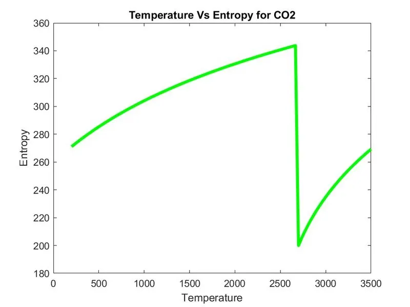
    title("Temperature Vs Entropy for " + speciesname)

    %Saving
    cd(['C:\Users\Naveen Kannan\Documents\MATLAB\Nasa Thermo\',speciesname]);

    saveas(1,'T VS Specific_Heat','jpg')
    saveas(2,'T VS Enthalpy','jpg')
    saveas(3,'T VS Entropy','jpg')


      %Molecular Weight calculation

      %Set of predominant Atoms in the dat file and their Atomic Weights
      %taken from periodic table
      Atoms = {'H' 'C' 'O' 'N' 'AR'};
      Atomic_Wt = [1 12 16 14 40];

      mol_wt = 0;
      %comparing the species name with the set of atoms
      for m = 1:length(speciesname)
          for n = 1:length(Atoms)
            if strcmp(speciesname(m),Atoms(n))
                mol_wt = mol_wt + Atomic_Wt(n);
                position = n;
            end
          end
          num_val = str2double(speciesname(m));
          if num_val > 1
              mol_wt = mol_wt + Atomic_Wt(position)*(num_val-1);
          end
      end

      if (strcmp(speciesname,Atoms(5)))
          mol_wt = mol_wt + Atomic_Wt(5);
      end

      %Displaying the final value of molecular weight in command window
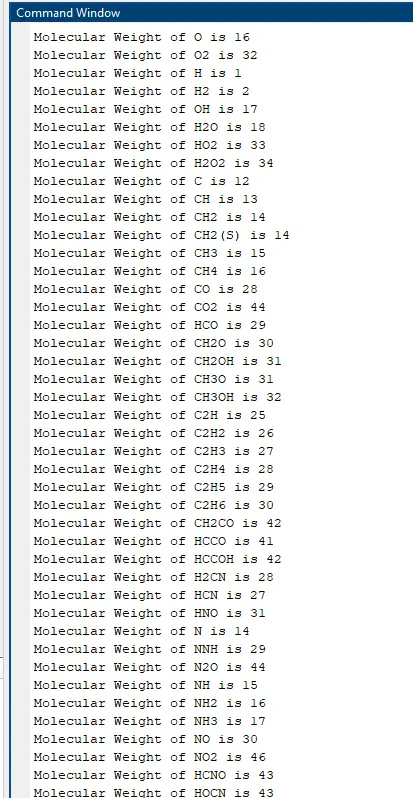
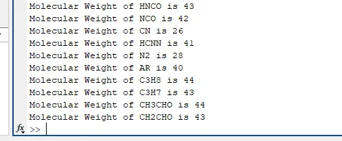
      disp("Molecular Weight of " + speciesname + " is " + mol_wt)

end
Screenshot of Folder

All Plots for O2
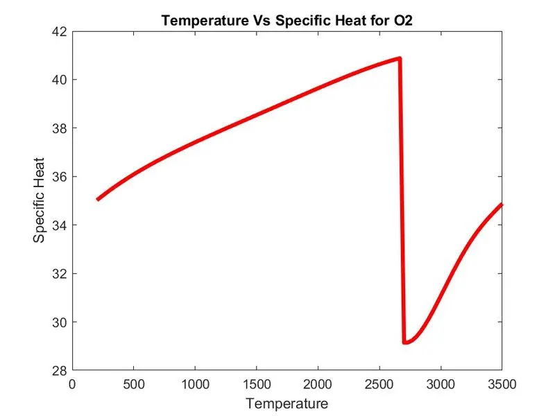
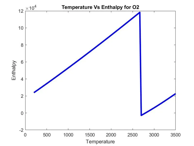
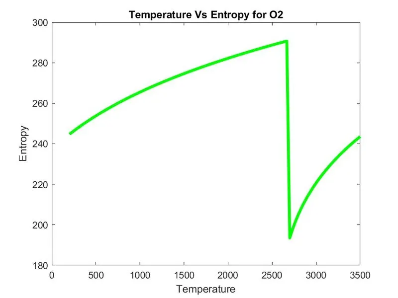
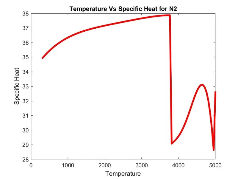
All Plots for N2
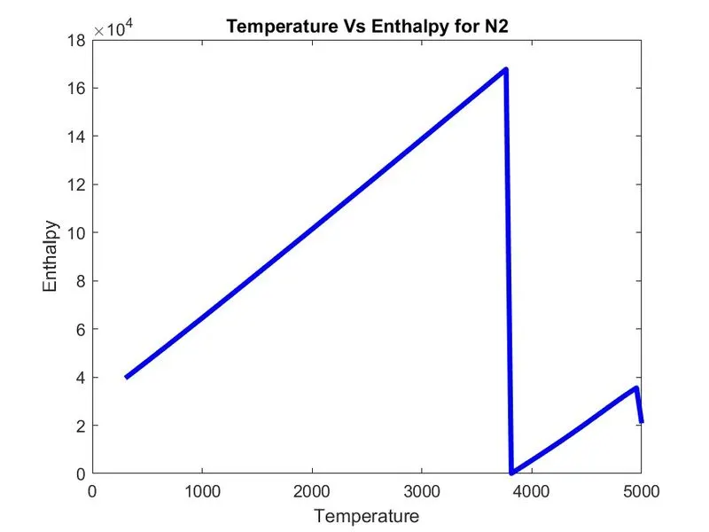
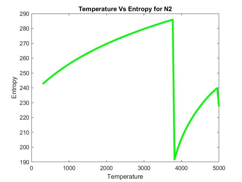
All Plots for CO2
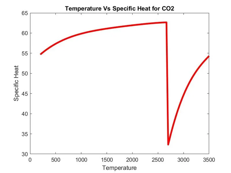
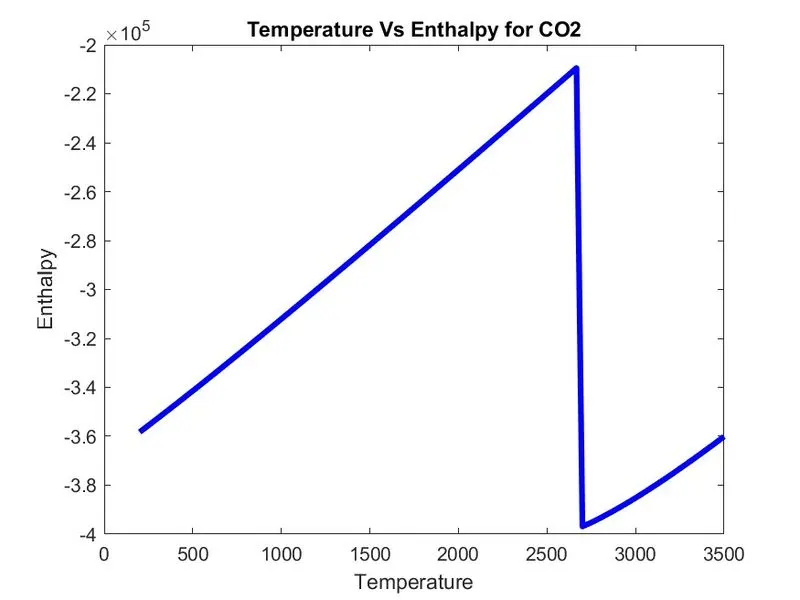
Command Window screenshot for molecular weight
Aim:
Write a program to parse a given file, extract the data and to calculate thermodynamic properties.
Equations Used:
Specific Heat Cp:
`C_p/R =a_1+ a_2×T + a_3×T^2 + a_4×T^3 + a_5×T^4`
Enthalpy H:
`H/(RT)= a_1+ (a_2×T)/2+(a_3×T^2)/3+ (a_4×T^3)/4+ (a_5×T^4)/5 + a_6/T`
Entropy S:
`S/R= a_1 lnT+ a_2×T +(a_3×T^2)/2 + (a_4×T^3)/3 + (a_5×T^4)/4 + a_7`
Explanation:
Stage 1:
%------------------Project-1 File Parsing----------------------------------
%---------- Parsing NASA thermodynamic data--------------------------------
%------Calculating Cp, H, S and Plotting in graph vs Temp.-----------------
%--------------Saving each species in each respective folder---------------
clear
close
clc
%Parsing Data file
file_read = fopen('THERMO.dat','r');
%Skipping the first 5 lines
for i = 1:5
fgetl(file_read);
end
- First the given file is opened in MATLAB.
- MATLAB has in-built commands for file handling. Here ‘fopen’ is used.
- This will instruct the MATLAB to open the file.
- Since fopen command also needs to be specified with the file access mode, so ‘r’ is specified to access the file in read mode.
- After, the file has been read the next is to take each line to extract the values.
- For getting each line ‘fgetl’ command is used.
- Each time when fgetl is called it would return the new line only as character array.
- Since, the first 5 lines in the file is not of purpose they can be skipped.
Stage 2:
%getting data for 53 species
for j = 1:53
%getting data of species specimen
line_1 = fgetl(file_read);
str_line = strsplit(line_1,' ');
speciesname = str_line{1};
%local temperatures
low_temp = str2double(str_line{end-3});
high_temp = str2double(str_line{end-2});
mid_temp = str2double(str_line{end-1});
%co-efficients
%high temp co-eff. a1 to a5
%co-eff 1 to 5 at line 2
line_2 = fgetl(file_read);
pos1 = strfind(line_2,'E');
a1 = str2double(line_2(1:pos1(1)+3));
a2 = str2double(line_2(pos1(1)+4:pos1(2)+3));
a3 = str2double(line_2(pos1(2)+4:pos1(3)+3));
a4 = str2double(line_2(pos1(3)+4:pos1(4)+3));
a5 = str2double(line_2(pos1(4)+4:pos1(5)+3));
%co-eff 6 to 10 at line 3
line_3 = fgetl(file_read);
pos2 = strfind(line_3,'E');
%high temp co-eff. a6 to a7
a6 = str2double(line_3(1:pos2(1)+3));
a7 = str2double(line_3(pos2(1)+4:pos2(2)+3));
%low temp co-eff. a8 to a10
a8 = str2double(line_3(pos2(2)+4:pos2(3)+3));
a9 = str2double(line_3(pos2(3)+4:pos2(4)+3));
a10 = str2double(line_3(pos2(4)+4:pos2(5)+3));
co-eff 11 to 14 at line 4
line_4 = fgetl(file_read);
pos3 = strfind(line_4,'E');
%low temp co-eff. a11 to a14
a11 = str2double(line_4(1:pos3(1)+3));
a12 = str2double(line_4(pos3(1)+4:pos3(2)+3));
a13 = str2double(line_4(pos3(2)+4:pos3(3)+3));
a14 = str2double(line_4(pos3(3)+4:pos3(4)+3));
- After, skipping the lines, next the data of the specimens needs to be extracted using the ‘fgetl’ command.
- As the fgetl command returns the line as character array it needs to be split to get the useful information.
- Once the line is split it is of a cell array. With the indexing technique extract the data that is needed.
- Species name, Low, High and Mid temperatures and the temperature co-efficients.
- For the data that is needed in number format ‘str2double’ command is used.
- From the file there are 14 temperature co-efficients the first 7 are high temperature co-efficients, and the next 7 are low temperature co-efficients.
Stage 3:
%Calculation of Cp,H,S
T = linspace(low_temp,high_temp,100);
for in = 1:length(T)
t = T(in);
if(t<=mid_temp)
T1(in) = t;
else
T2(in) = t;
end
end
ltr = T1;
htr = T2((length(ltr)+1):end);
%gas const.
R = 8.314;
%Cp, H , S at htr
%htr coeff a1 to a7
cp1 = (a1 + (a2*htr) + (a3*htr.^2) + (a4*htr.^3) + (a5*htr.^4))*R;
h1 = (a1 + ((a2*htr)/2) + ((a3*htr.^2)/3) + ((a4*htr.^3)/4) + ((a5*htr.^4)/5) + (a6./htr))*R.*htr;
s1 = ((a1*log(htr)) + (a2*htr) + ((a3*htr.^2)/2) + ((a4*htr.^3)/3) + ((a5*htr.^4)/4) + a7)*R;
%Cp, H, S at ltr
%ltr coeff a8 to a14
cp2 = (a8 + (a9*ltr) + (a10*ltr.^2) + (a11*ltr.^3) + (a12*ltr.^4))*R;
h2 = (a8 + ((a9*ltr)/2) + ((a10*ltr.^2)/3) + ((a11*ltr.^3)/4) + ((a12*ltr.^4)/5) + (a13./ltr))*R.*ltr;
s2 = ((a8*log(ltr)) + (a9*ltr) + ((a10*ltr.^2)/2) + ((a11*ltr.^3)/3) + ((a12*ltr.^4)/4) + a14)*R;
Cp = [cp1,cp2];
H = [h1,h2];
S = [s1,s2];
%Creating folder
mkdir(['C:\Users\Naveen Kannan\Documents\MATLAB\Nasa Thermo\',speciesname]);
%Plotting
figure(1)
plot(T,Cp,LineWidth=3,Color='r')
xlabel('Temperature')
ylabel('Specific Heat')
title("Temperature Vs Specific Heat for " + speciesname)
figure(2)
plot(T,H,LineWidth=3,Color='b')
xlabel('Temperature')
ylabel('Enthalpy')
title("Temperature Vs Enthalpy for " + speciesname)
figure(3)
plot(T,S,LineWidth=3,Color='g')
xlabel('Temperature')
ylabel('Entropy')
title("Temperature Vs Entropy for " + speciesname)
%Saving
cd(['C:\Users\Naveen Kannan\Documents\MATLAB\Nasa Thermo\',speciesname]);
saveas(1,'T VS Specific_Heat','jpg')
saveas(2,'T VS Enthalpy','jpg')
saveas(3,'T VS Entropy','jpg')
- After extracting all data that is needed, the next step is to calculate the specific heats, enthalpy and entropy.
- Since there are three temperatures, with a mid-value, temperature array is defined using ‘linspace’ command with the low and high temperatures extracted and the values are compared with the mid-temperature and is split into two regions namely low and high.
- With the given formulae for specific heat, enthalpy and entropy can be calculated for these two regions by substituting the temperature co-efficients accordingly.
- So, there will be two sets of each properties calculated one is for high temperature region and the other for low temperature region.
- These are combined as single entity and is plotted vs temperature.
- All the plots are saved into the folder directly.
- ‘mkdir’ command is used to create a folder in the name of the species extracted.
- ‘cd’ command is used to change the current folder to the created folder.
- ‘saveas’ command is used to save the figures as the format needed.
Stage 4:
%Molecular Weight calculation
%Set of predominant Atoms in the dat file and their Atomic Weights
%taken from periodic table
Atoms = {'H' 'C' 'O' 'N' 'AR'};
Atomic_Wt = [1 12 16 14 40];
mol_wt = 0;
%comparing the species name with the set of atoms
for m = 1:length(speciesname)
for n = 1:length(Atoms)
if strcmp(speciesname(m),Atoms{n})
mol_wt = mol_wt + Atomic_Wt(n);
position = n;
end
end
num_val = str2double(speciesname(m));
if num_val > 1
mol_wt = mol_wt + Atomic_Wt(position)*(num_val-1);
end
en the d
if (strcmp(speciesname,Atoms(5)))
mol_wt = mol_wt + Atomic_Wt(5);
end
%Displaying the final value of molecular weight in command window
disp("Molecular Weight of " + speciesname + " is " + mol_wt)
end
- The next is to calculate the molecular weights of each species.
- The atomic weights of each atoms in the species is taken from the periodic table as an array.
- With these atomic weight values, the molecular weights are calculated.
- ‘disp’ command used to display in the command window.
Error:
There were no significant errors during execution and coding.