Week 3 - Solving second order ODEs

%--------------------Week 3 - challenge-------------------------------------------------
%-----------Solve the ODE to get the movement of the pendulum---------------------------
clear all 
close all
clc

L = 1;
m = 1;
b = 0.05;
g = 9.81;

%initial condition
theta_0 = [0;3];

%time points
time_span_motion = linspace(0,20,500);

%solve ODE
[t, results] = ode45(@(t, theta) ode_chal(t,theta,b,g,L,m),time_span_motion,theta_0);


plot(t,results(:,1))
hold on
plot (t,results(:,2))
ylabel('ang. Disp. &  ang. Velocity')
xlabel('Time in s')
%----------Animation-----------------------
counter = 1;
X0 = 0;
Y0 = 0;
for i=1:length(t)
    X1 = L*sin(results(i,1));
    Y1 = -L*cos(results(i,1));

    figure(2)
    plot([-1 1],[0 0],'LineWidth',4, 'Color','black')
    axis([-2 2 -2 2])
    line([X0 X1],[Y0 Y1],'LineWidth',3,'color','g')
    hold on
    plot(X0,Y0,'Marker','*','MarkerSize',3,'MarkerFaceColor','r')
    plot(X1,Y1,'Marker','o','MarkerSize',10,'MarkerFaceColor','blue')
    grid on
    hold off
    M(counter) = getframe(gcf);
    counter = counter+1;
end

movie(M)
videofile = VideoWriter('pendulum_animation challenge.mp4','MPEG-4');
open(videofile)
writeVideo(videofile,M)
close(videofile)

----------------------------------------------------------------------------------------
---------------------------function - Supplement----------------------------------------
function [dtheta_dt] = ode_chal(t,theta,b,g,L,m)

theta1 = theta(1);
theta2 = theta(2);

dtheta1_dt = theta2;
dtheta2_dt = -(b/m)*theta2-(g/L)*sin(theta1);

dtheta_dt = [dtheta1_dt ;dtheta2_dt];
end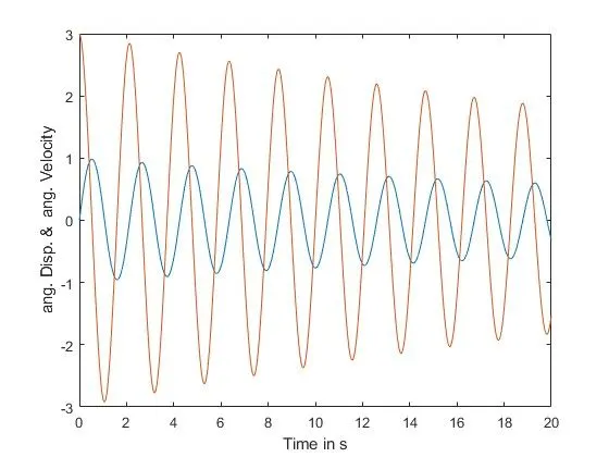

Aim:

To write a program that solves a 2^nd order Ordinary Differential Equation to compute the damping and motion of a simple pendulum and to animate it.

2^nd order Ordinary Differential Equation:

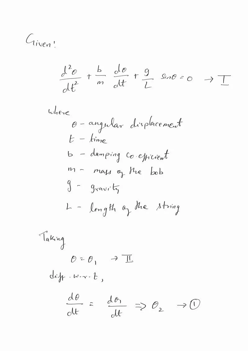
`(d^2 θ)/dt^2 + b/m (dθ)/dt+g/L sin⁡θ=0`

, is the differential equation of a simple pendulum with damping.

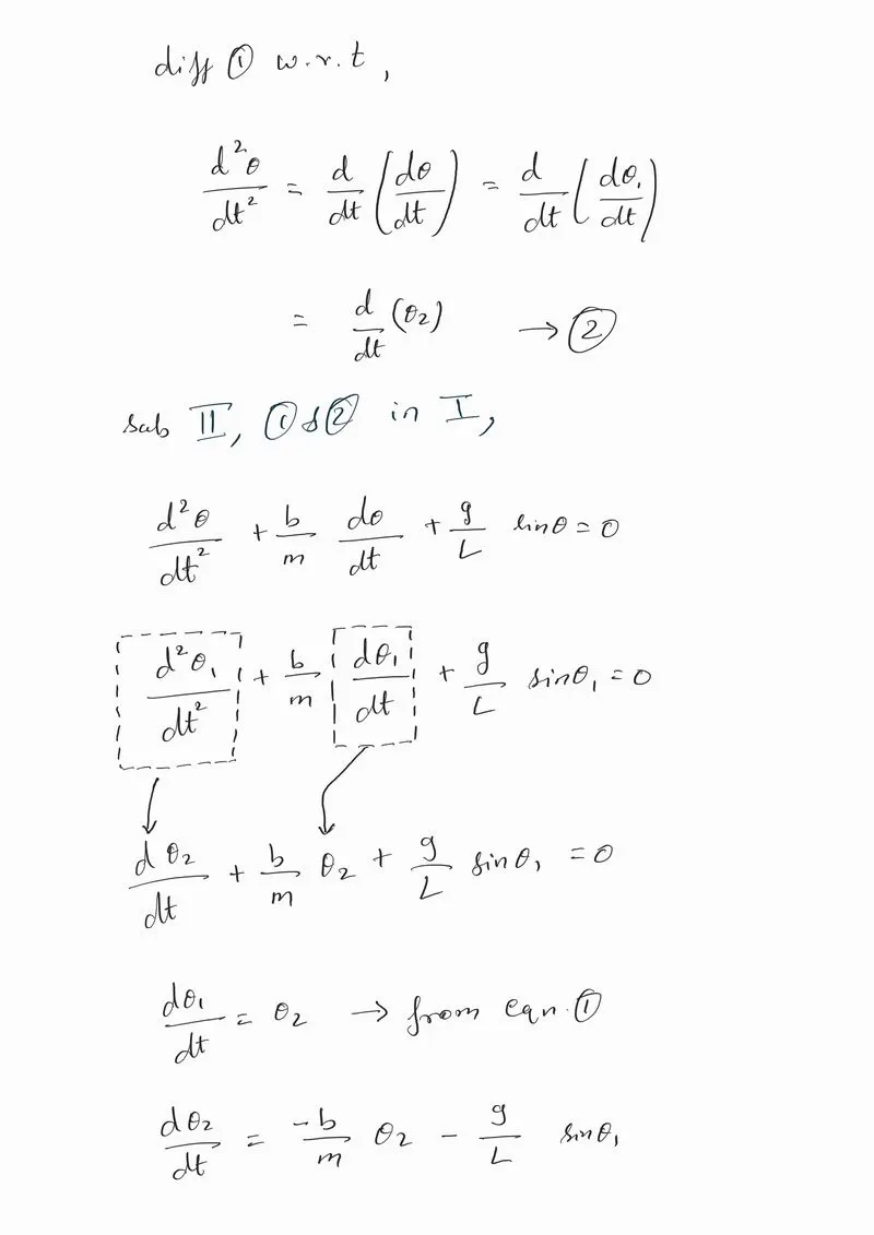
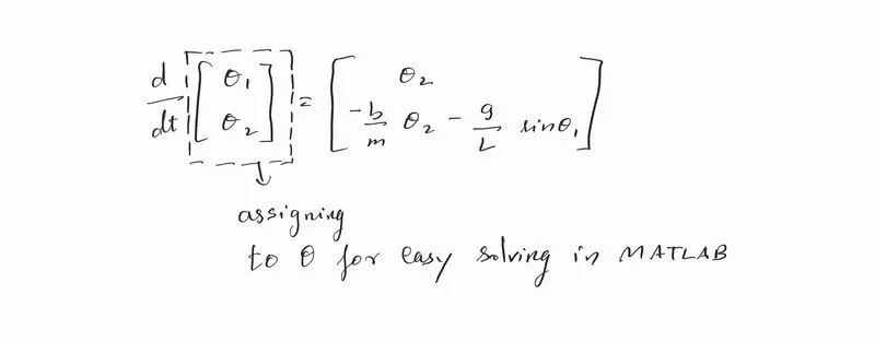
Generally, a higher order differential equation can be split into a simultaneous system of lower order differential equations in order to solve it quickly and easily. In this case, since it is a 2^nd order, we can split it up into 2 simultaneous 1^st order which is given below.

Problem Statement:

Simulate the motion between 0-20 sec, for angular displacement=0, angular velocity=3 rad/sec at time t=0.

Given,

L=1 m,

m=1 kg,

b=0.05.

g=9.81 m/s2.

Solving 2^nd order ODE:

Explanation:

Stage 1:

%--------------------Week 3 - challenge------------------------------------

%-----------Solve the ODE to get the movement of the pendulum--------------

clear all

close all

clc

L = 1;

m = 1;

b = 0.05;

g = 9.81;

%initial condition

theta_0 = [0;3];

%time points

time_span_motion = linspace(0,20,500);

%solve ODE

[t, results] = ode45(@(t, theta) ode_chal(t,theta,b,g,L,m),time_span_motion,theta_0);

plot(t,results(:,1))

hold on

plot (t,results(:,2))

ylabel('ang. Disp. & ang. Velocity')

xlabel('Time in s')

• The variables for mass, length, gravity, damping co-eff. are declared and initialized.
• Since the problem statement states that simulate the motion between 0 and 20 seconds, the time span is given as a linear vector that has values between 0 & 20 with 500 instances for smooth and better visuals.
• Then we need the initial conditions which also given in the statement as angular displacement = 0 and angular velocity = 3rad/s at time t=0.
• Declaring these initial conditions and time span as given below,
  • %initial condition

theta_0 = [0;3];

is the initial condition of the ODE, the semicolon ‘;’ inside the brackets specifies and instructs the MATLAB to initialize this as a column vector/ column matrix where the 1^st row is the initial condition of angular displacement and the 2^nd row is the initial condition of angular velocity.

• %time points

time_span_motion = linspace(0,20,500);

is the time span in which the change in ang. Disp. and ang. Velocity are been calculated and the motion is generated. The ‘linspace’ command instructs the MATLAB to create a row vector between 0 & 20 with 500 instances.

• The next step is to solve the ODE, MATLAB has an in-built ODE solver that solves and integrates the ODE with these given conditions provided.

[t, results] = ode45(@(t, theta) ode_chal(t,theta,b,g,L,m),time_span_motion,theta_0);

• [t, results] is the final solution matrix from the ODE solver.
• ode45 is the name of the in-built solver.
• @(t,theta) instructs and specifies that the given ODE is a function of t and theta.
• ode_chal(t,theta,b,g,L,m) is the supplement function name that returns the solution vector ‘dtheta_dt’ which is ‘results’ in [t,results] of the final solution. This function takes inputs like time span, initial conditions, mass, length, gravity and the damping co-eff., from the main program.
• time_span_motion is the limits for the ODE which is used to find the ang. Disp., and ang. Velocities at all the ‘500’ time instances.
• theta_0 is the initial conditions.

• Once the final solution matrix is found the next is to plot ang.Disp., and ang.Velocity against time.
  • For this ‘plot’ command is used to plot the curves and hence MATLAB executes only the latest plot command and shows the figure, we use ‘hold on’ that instructs MATLAB to hold the same figure to plot all the curve that we specify.
  • For time vs ang.Disp. plot time ‘t’ and ang.Disp. column from the ‘results’ from the final solution matrix.
  • For time vs ang.Velocity plot time ‘t’ and ang.Velocity column from the ‘results’ from final solution matrix.

ODE Function – Supplement:

function [dtheta_dt] = ode_chal(t,theta,b,g,L,m)

theta1 = theta(1);

theta2 = theta(2);

dtheta1_dt = theta2;

dtheta2_dt = -(b/m)*theta2-(g/L)*sin(theta1);

dtheta_dt = [dtheta1_dt ;dtheta2_dt];

end

• This function supplements the main program that solves the system of ODEs and throws the output results.
• Here dtheta_dt is the result/solution vector that is given as output.

`(dθ)/dt= d/dt [■(θ_1@θ_2 )]`

• Since, MATLAB handles only matrixes for storing and performing operations we are specifying the variables in matrix form.
• Function takes the input parameters mass, damping co-efficient, length, time, and the initial conditions of the ODE àangular displacement and angular velocity and gives out the result with series of angular displacements and angular velocities which in other words gives the position and speed of the pendulum with respect to time.

Stage 2:

%----------Animation-----------------------

counter = 1;

X0 = 0;

Y0 = 0;

for i=1:length(t)

X1 = L*sin(results(i,1));

Y1 = -L*cos(results(i,1));

figure(2)

plot([-1 1],[0 0],'LineWidth',4, 'Color','black')

axis([-2 2 -2 2])

line([X0 X1],[Y0 Y1],'LineWidth',3,'color','g')

hold on

plot(X0,Y0,'Marker','*','MarkerSize',3,'MarkerFaceColor','r')

plot(X1,Y1,'Marker','o','MarkerSize',10,'MarkerFaceColor','blue')

grid on

hold off

M(counter) = getframe(gcf);

counter = counter+1;

end

movie(M)

videofile = VideoWriter('pendulum_animation challenge.mp4','MPEG-4');

open(videofile)

writeVideo(videofile,M)

close(videofile)

• The next step is to make an animation of the motion of the pendulum with the obtained data.
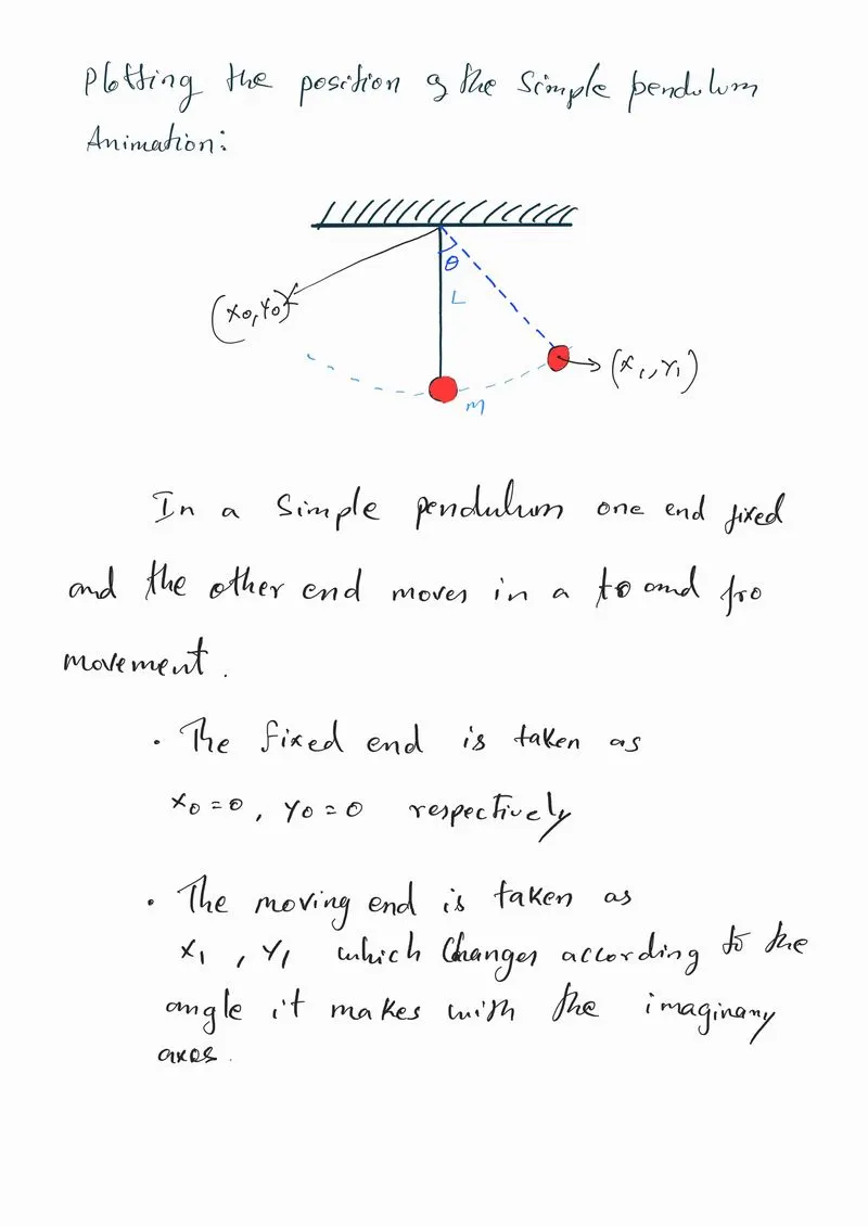
• To plot the position of the pendulum we need to figure out the free body diagram of the pendulum, which is given below.

• The counter variable is used for stitching the figures to make a movie.
• The origin points are declared and initialized with X0, Y0 which is also the fixed end of the pendulum.
• From the final solution matrix the ‘results’ matrix contains the data of ang.Disp and ang.Velocity for ‘500’ time instances.
• We know the length of the string of the pendulum as L=1.
• With these data we can calculate the position of the free/moving end of the pendulum.
• Since the time of 20 seconds is given with 500 instances, we initialize the time ‘t’ in a for loop starting from 1^st instance and iterates upto the last instance.
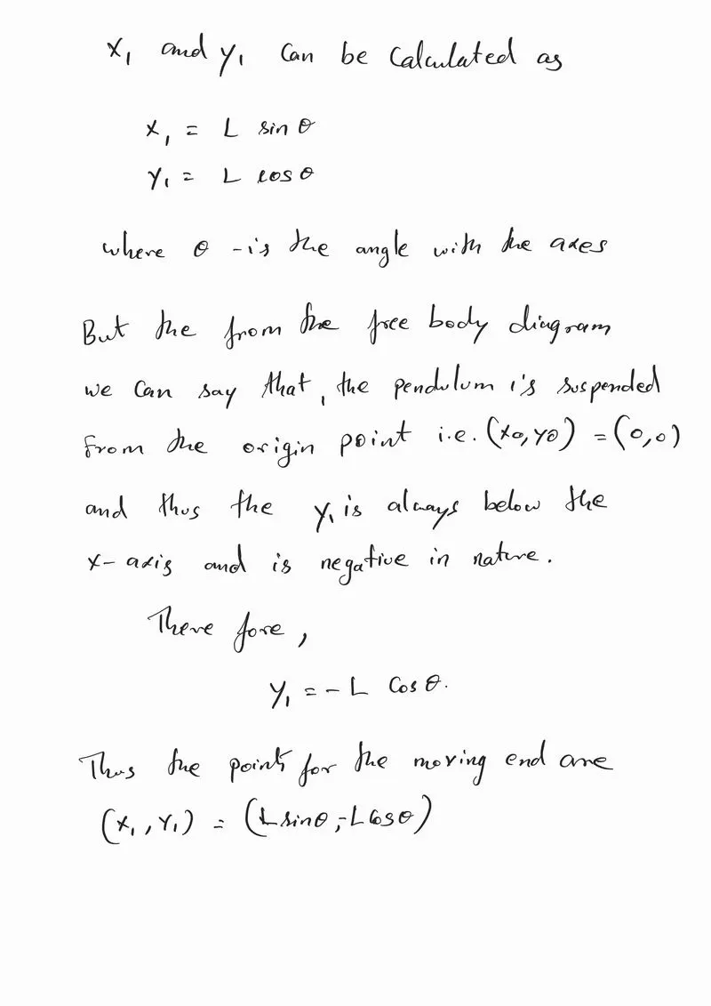
• Inside the loop we can calculate the position of the free end with name X1 & Y1.
• The formula for calculating X1 & Y1 are,
  • X1 = L*sin(results(i,1))
  • Y1 = - L*cos(results(i,1))
• The ‘results’ matrix contains the ‘ang.Disp’ in the first column and the ‘ang.Velocity’ in the second column. But we need only the disp. values, so we take only the values in column 1 at each instance ‘i’ of the time span.
• After calculating the X1 & Y1 values we can proceed for plotting them.
  • To plot we can open a new figure with ‘figure (2)’ command, since the figure 1 is already being used for the earlier plots.
  • Plot a line which would represent the fixed axis in which the pendulum is being suspended.
  • Plot a line which represents the string of the pendulum, here the points X0 to X1 and Y0 to Y1 is used with the ‘line’ command.
  • To plot the suspended bob ‘sphere’ at the free end, ‘hold on’ command is used to instruct MATLAB to hold the same figure window.
  • To plot the fixed end the points at origin X0 & Y0 is plotted with ‘marker’ – “*”, here ‘marker’ command is used.
  • The same ‘marker’ command is used to specify the sphere bob also with its size and color.
  • Then ‘hold off’ command is used to instruct MATLAB to release the plot figure.
  • Then a variable M is declared and initialized with the ‘counter’ variable which captures the current figure frame.
  • And next the ‘counter’ is incremented by 1 each and everytime the for loop gets executed.
• After capturing all the plot figure frames ‘movie’ command is used to stitch the frames which are stored in the variable ‘M’.
• Then the video file needs to be created by ‘VideoWriter’ command passing the filename and the compression profile as parameters and assigning it to a variable.
• Then the videofile is opened, and the captured frames are written into the file using ‘writeVideo’ command by passing the video file variable and the stitched frames as parameters.
• Then the videofile is closed.
• The video file will be created in the directory/folder.

Errors Occurred:

While calculating the position of the free/moving end X1 & Y1, in Y1 I accidentally missed the ‘-‘ sign in front of the formula. When I ran the program, I got the figure of the pendulum above the fixed point. This is attached as video appended with error in the last of the filename.

Rectification:

I added the ‘-‘ sign in the Y1 formula and reran the program. This time it produced the desired result.

Vidoe files google drive link

file 1 ; https://drive.google.com/file/d/18Jl4I4GQsFrcI-oBvERWYaBJv6oY64nI/view?usp=sharing

file 2 ; https://drive.google.com/file/d/10seY1JbIDRMamTCJsEwtI2Yx10_h2Lm3/view?usp=sharing