Week 4.1 - Genetic Algorithm

Aim

To write a program to find global maxima in stalagmite function using solver ‘Genetic Algorithm’ in MATLAB.

Theory

--Optimisation

Optimisation is decision making process.
it is used to find the best results under a set of criteria or constraints. the procedure is executed iteratively by comparing various solutions till an optimum or satisfactory solution is found.

--Genetic algorithm
this is a type of optimisation process, It is a search based optimisation technique based on the principles of genetics and natural selection.It is frequently used to find optimal or near optimal solutions.

genetic algorithm oprtimisation starts with population initialization

in the initialisation, we have to decide the population size. higher the population size,we will get more combinations and more accurate results.
population is the number of sample data points(chromosomes) taken to perform the genetic algorithm operation.

-Selection

in this step, the parents are selected from the sample data points,main objectieve of the selection process is to select the highly fit individuals.The fitness value of the given function is computed, the fittest value will have most probablity to get selected.

-Cross over.

it is the process of taking two parents and producing teh childs from thm by interchanging the genes.

-Mutation

mutation is carried out to maintain the genetic diversity from one generation of a population of chromosomes to the next.

these three processes (SELECTION -> CROSSOVER -> MUTATION) are repeated for the new offspring by replacing the parents until an optimised result is found.

Fitness function is a function which measures how good the solution is. it takes the solution as input and produces the suitability of the solution as the output.This evaluates how close the solution is to the optimal solution of the desired problem

Genetic algorith is used in areas like Optimisation,Economics,Neural networks and Image processing.

--Syntax for GA

x=ga(fun,nvars,A,b,Aeq,beq,lb,ub,nonlcon,options)

fun= Objective function
nvar=Number of variables(specified as positive integer)
A,b=Linear inequality constraints(A= Real matrix,b=Real vector)
Aeq,beq=Linear equality constraints(A= Real matrix,b=Real vector)
Lb,ub=Lower bounds and upper bounds
nonlcon=Nonlinear constraints
options=Optimization options

--Significance of running Multiple iterations and cases

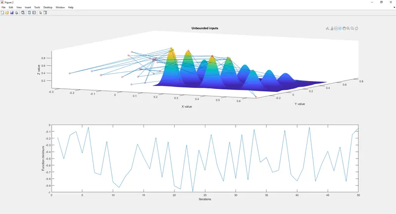
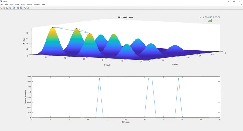
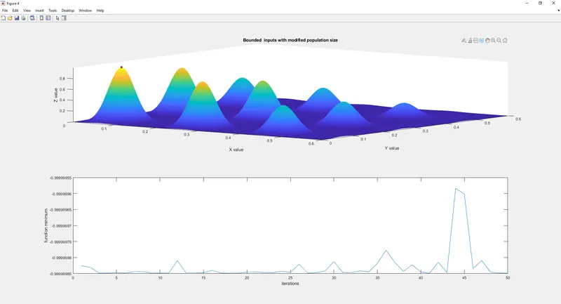
We can see how more data inputs give a better result. it is easier to choose the best fitted value with more constraints. at first we gave an unbounded case where lower and upper bounds not defined and we got more inaccurate results.In the next case we defined lower and upper bound values and we got better optimised results. in the third case we along with lower and upper bounds we changed the options of population size by using optimoptions which resulted in more accurate result.
we run GA multiple iterations to make sure if the uotput we are getting is stable or not.

--Stopping Criteria of GA

The Stopping Criteria is the different conditions we give to stop the genetic algorithm slover.

-MaxGenerations - The algorithm stops when the number of generations reaches Max generations
-MaxTime - The algorithm stops after running for an amount of time in seconds equal to MaxTime.
-FitnessLimit - The algorithm stops when the value of fitness function for the best point in the current population is less than or equal to FitnessLimit
-MaxStallGenerations- The algorithm stops when the average relative change in the fitness function value over MaxStallGenerations is less than function tolerance
-MaxStallTime - The algorithm stops if there is no improvement in the objective function during an interval of time in seconds equal to MaxStallTime
FunctionTolerance- The algorithm runs until the average relative change in the fitness function value over MaxStallGenerations is less than FunctionTolerance.

Stalagmite Function

function[f]= stalagmite1(inputs)

x=inputs(1)
y=inputs(2)

  f1x=(sin(5.1*pi*x+0.5))^6;
  f1y=(sin(5.1*pi*y+0.5))^6;

  f2x=exp((-4*log(2)*(((x-0.0667)^2)/0.64)));
  f2y=exp(-4*log(2)*(((y-0.0667)^2)/0.64));
  
  f=-(f1x*f1y*f2x*f2y);

  %GA is designed to give global minima so we use -ve sign
end

Main code

clear 
close
clc

x = linspace(0,0.6,150);
y = linspace(0,0.6,150);

num_cases = 50;

[xx, yy] = meshgrid(x, y);

for i = 1:length(x)
    for j = 1:length(y)
        inputs(1)=xx(i,j);
        inputs(2)=yy(i,j);
        f(i,j) = stalagmite1(inputs);
    end
end
figure(1)
surfc (xx,yy,-f);
xlabel( 'X value')
ylabel( 'Y value')
zlabel('Z value')
title('Basic surface plot')
shading interp

%Study 1 Statistical behaviour
tic
for i= 1:num_cases
    [inputs, fopt(i)] = ga(@stalagmite1, 2);
    xopt(i) = inputs(1);
    yopt(i) = inputs(2);
end
study1_time = toc;

figure(2)
subplot(2,1,1)
hold on
surfc(x,y,-f)
shading interp
plot3(xopt,yopt,-fopt,'marker','o','MarkerSize',5,'MarkerEdgeColor','r')
title('Unbounded inputs')
xlabel( 'X value')
ylabel( 'Y value')
zlabel('Z value')
subplot(2,1,2)
plot(fopt)
xlabel('Iterations')
ylabel('Function minimum')

tic
%Study 2 Statistical behaviour with upper and lower bounds

for i=1:num_cases
    [inputs,fopt(i)] = ga(@stalagmite1,2,[],[],[],[],[0;0],[0.4;0.4]);
    xopt(i) = inputs(1);
    yopt(i) = inputs(2);
end
study2_time = toc;

figure(3)
subplot(2,1,1)
hold on
surfc(x, y,-f)
shading interp
plot3(xopt,yopt,-fopt,'marker','o','markersize',5,'MarkerFaceColor','r')
title('Bounded  inputs')
xlabel( 'X value')
ylabel( 'Y value')
zlabel('Z value')
subplot(2,1,2)
plot(fopt)
xlabel('iterations')
ylabel('function minimum')

%Study 3 increasing GA iterations
options = optimoptions('ga');
options =optimoptions(options,'PopulationSize',270);

tic
for i =1:num_cases
    [inputs,fopt(i)] =ga(@stalagmite1,2,[],[],[],[],[0;0],[0.4;0.4],[],[],options);
    xopt(i) = inputs(1);
    yopt(i) = inputs(2);
end
study3_time = toc;

figure(4)
subplot(2,1,1)
hold on
surfc(x, y,-f)
shading interp
plot3(xopt,yopt,-fopt,'marker','o','markersize',5,'MarkerFaceColor','r')
title('Bounded  inputs with modified population size')
xlabel( 'X value')
ylabel( 'Y value')
zlabel('Z value')
subplot(2,1,2)
plot(fopt)
xlabel('iterations')
ylabel('function minimum')

Step-wise explanation of code

Lower and upper limit is set and array of values within the limit is taken with the linspace() command
the number of cases is set to be 50

nested for loop is made for the input array to be called simultaneously for the stalgmite function

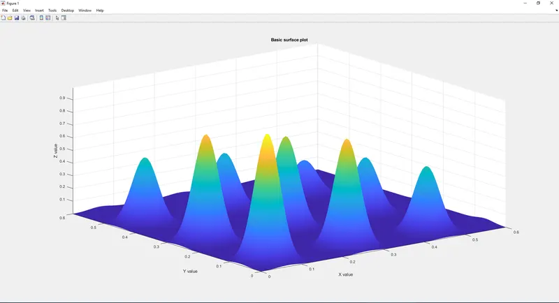
surface plot is created with surfc() command we gave f negative value because GA is designed to give global minima
the shading interp command is used for better look of the surface plot without the outlines

in the first case we use genetic algorithm with unbounded inputs. which means we only gave the user defined function
stalgmite1 and the number of variables(2) as input to the inbuilt function ga(). a tic- toc command is used to note time taken for the function to run.

this ga is run inside a for loop since we have to run all the inputs for x and y

the unbounded ga function is plotted into two subplots, one which is the surface with the genetic selection is shown and the other in a graph with iterations and function minimum

in the surface subplot, we used the plot3() command to show the selection process

similar procedures are done in the second and third studies only differences are;

in the second case we defined lower and upper bound values as [0;0] and [0.4;0.4] we gave null brackets [] where other inputs like Linear inequality constraints,Linear equality constraints should be given since we are not defining those values.
in the third case along with the constraints given in the second conditon,we modified one option with the optimoptions() function which is used to Create/modify optimization options. we modified PopulationSize to 270 to get a wider range and better fitness.

both 2 & 3 cases are plotted as the first case

Outputs

Surface plot with given range of arrays

Genetic algorithm with unbounded inputs

Genetic algorithm with lower and upper bound values defined

Genetic algorithm with lower and upper bound values defined and modified population size of 270

Error faced

Gave wrong function name in the main code 

References : Genetic Algorithm explained