Project 2 - Rankine cycle Simulator

Aim

To simulate the Rankine Cycle and plot the corresponding T-S and H-S plots using MATLAB.

Objective

Calculate the state points of the Rankine Cycle based on given inputs.
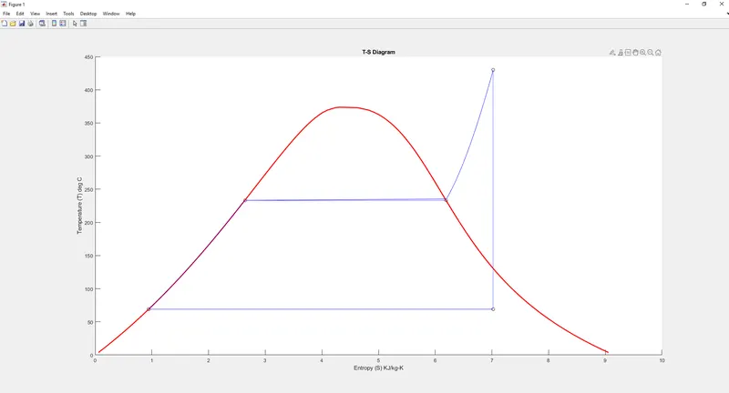
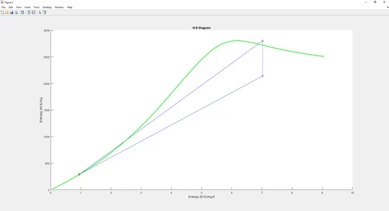
Plot the corresponding T-S and H-S plots for the given set of inputs.

Theory

Rankine Cycle:
It is a model which is used to predict the performance of steam turbine systems. It is a thermodynamic cycle of a heat engine that converts heat into mechanical work while undergoing phase change.

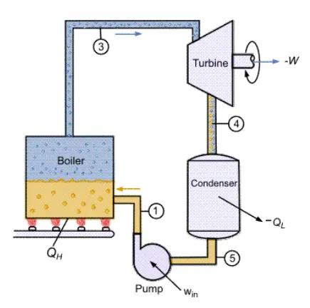
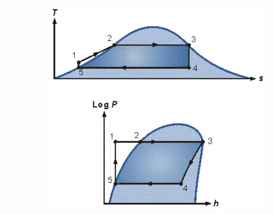
Rankine Cycle Process:

1-3 Isobaric Heat Transfer:

In this process, a high pressure liquid enters the boiler from the feed pump. This liquid is heated to the saturation temperature. It is heated to form vapour i.e. evaporation takes place and the saturated steam is formed.

3-4 Isentropic Expansion:

In this process, the vapour is expanded in the turbine, this produces mechanical work which will be converted to electricity.

4-5 Isobaric Heat Rejection:

In this process, the vapour-liquid mixture leaving the turbine is condensed at low pressure, usually in a surface condenser using cooling water.

5-1 Isentropic Compression:

In this process, the pressure of the liquid is raised in the feed pump. Because of the low specific volume of liquids, the pump work is relatively small and often neglected in thermodynamic calculations.

Input Values

Turbine Inlet temperature = 400° C
Turbine Inlet Pressure = 30 bars
Turbine Outlet Pressure = 0.05 bars = Condenser Inlet Pressure

Required Output Values:

Net work output
Back work ratio

Main Code

%Rankine Cycle Simulator
clear all
close all
clc

fprintf('\n')
disp(' Rankine Cycle Simulator ')

%Rankine Cycle Processes
fprintf('\n')
disp('1-2 Isentropic compression')
disp('2-3 Isobaric heat addition')
disp('3-4 Isentropic expansion')
disp('4-1 Isobaric heat rejection')

%Values for saturation curves
Temp_ts_s= linspace(0,373,100);

for i = 1:length(Temp_ts_s)
    entr_l(i) = XSteam('sl_t',Temp_ts_s(i));
    entr_v(i) = XSteam('sv_t',Temp_ts_s(i));
end
for i = 1:length(Temp_ts_s)
    enth_l(i) = XSteam('hl_t',Temp_ts_s(i));
    enth_v(i) = XSteam('hv_t',Temp_ts_s(i));
end

%Values of critical point of water
Temp_c = 373.706;
Pressure_c = 220;
entr_c = XSteam('s_pt',Pressure_c,Temp_c);
enth_c = XSteam('h_ps',Pressure_c,entr_c);

%Values of H,S,P & T of saturated vapour at boiler outlet
fprintf('\n')
Temp_3 = input('Enter the temperature at turbine inlet (in deg C)= ');
Pressure_3 = input('Enter the pressure at turbine inlet (in bar)= ');
enth_3 = XSteam('hV_p',Pressure_3);
entr_3 = XSteam('s_pT',Pressure_3,Temp_3);

%Values of H,S,P & T of saturated vapour at turbine outlet
P_4 = input('Enter the pressure at condenser inlet (in bar)= ');
S_4 = entr_3;
H_4 = XSteam('h_ps',P_4,S_4);
gamma = 1.4;
T_4 = Temp_3*((P_4/Pressure_3)^(1-(1/gamma)));

%Values of H,S,P & T of saturated liquid at condenser outlet
Temp_1 = T_4;
Pressure_1 = P_4;
enth_1 = XSteam('hL_T',Temp_1);
entr_1 = XSteam('sL_T',Temp_1);

%Values of H,S,P & T of saturated liquid at pump outlet
entr_2 = entr_1;
Pressure_2 = Pressure_3;
enth_2 = XSteam('h_ps',Pressure_2,entr_2);
Temp_2 = XSteam('t_ps',Pressure_2,entr_2);

%Values of H,S,P & T for the subcooled liquid region
Pressure_22 = Pressure_3;
entr_22 = XSteam('sL_p',Pressure_22);
enth_22 = XSteam('h_ps',Pressure_22,entr_22);
Temp_22 = XSteam('T_hs',enth_22,entr_22);
Temp_sub = linspace(Temp_2,Temp_22,100);
for i = 1:length(Temp_sub)
    entr_sub(i) = XSteam('s_pT',Pressure_22,Temp_sub(i));
end

%Values of H,S,P & T for the superheated vapour region
S_33 = XSteam('sV_t',Temp_22);
T_33 = Temp_22;
T_sup = linspace(T_33,Temp_3,100);
for i = 1:length(T_sup)
    entr_sup(i) = XSteam('s_pT',Pressure_3,T_sup(i));
end

%values of thermal efficiency, specific steam consumption and back work ratio

W_Turbine = (enth_3 - H_4);
W_Pump = (enth_2 - enth_1);
W_Net = W_Turbine - W_Pump;
Q_Input = (enth_3 - enth_2);
Therm_Eff = (W_Net/Q_Input)*100;
SSC = (3600/W_Net);
BWR = W_Pump/W_Turbine;

%H-S and T-S graph plotting
figure(1);
hold on;
plot(entr_1,Temp_1,'o','color','k');
plot(entr_2,Temp_2,'o','color','k');
plot(entr_22,Temp_22,'o','color','k');
plot(S_33,T_33,'o','color','k');
plot(entr_3,Temp_3,'o','color','k');
plot(S_4,T_4,'o','color','k');

plot(entr_l,Temp_ts_s,'color','r','linewidth',2);
plot(entr_v,Temp_ts_s,'color','r','linewidth',2);
plot([entr_c entr_v(1,100)],[Temp_c Temp_ts_s(1,100)],'color','r','linewidth',2);
plot([entr_c entr_l(1,100)],[Temp_c Temp_ts_s(1,100)],'color','r','linewidth',2);

plot([entr_3 S_4],[Temp_3 T_4],'color','b');
plot([entr_1 S_4],[Temp_1 T_4],'color','b');
plot([entr_1 entr_2],[Temp_1 Temp_2],'color','b');
plot([entr_22 S_33],[Temp_22 T_33],'color','b');
plot(entr_sub,Temp_sub,'color','b');
plot(entr_sup,T_sup,'color','b');
xlabel('Entropy (S) KJ/kg-K');
ylabel('Temperature (T) deg C');
title('T-S Diagram');

figure(2);
hold on;
plot(entr_1,enth_1,'o','color','k');
plot(entr_2,enth_2,'o','color','k');
plot(entr_3,enth_3,'o','color','k');
plot(S_4,H_4,'o','color','k');

plot([entr_3 S_4],[enth_3 H_4],'color','b');
plot([entr_1 entr_2],[enth_1 enth_2],'color','b');
plot([entr_2 entr_3],[enth_2 enth_3],'color','b');
plot([entr_1 S_4],[enth_1 H_4],'color','b');

plot(entr_l,enth_l,'color','g','linewidth',2);
plot(entr_v,enth_v,'color','g','linewidth',2);
plot([entr_c entr_v(1,100)],[enth_c enth_v(1,100)],'color','g','linewidth',2);
plot([entr_c entr_l(1,100)],[enth_c enth_l(1,100)],'color','g','linewidth',2);
xlabel('Entropy (S) KJ/kg-K');
ylabel('Enthalpy (H) KJ/kg');
title('H-S Diagram');


%Printing the values of all state points and performance parameters
fprintf('\n')
disp(' Results ')
fprintf('\n At State point 1:')
fprintf('\n P1 is : %d bar',Pressure_1)
fprintf('\n T1 is : %d deg C',Temp_1)
fprintf('\n H1 is : %d KJ/kg',enth_1)
fprintf('\n S1 is : %d KJ/kg-K',entr_1)

fprintf('\n')
fprintf('\n At State point 2:')
fprintf('\n P2 is : %d bar',Pressure_2)
fprintf('\n T2 is : %d deg C',Temp_2)
fprintf('\n H2 is : %d KJ/kg',enth_2)
fprintf('\n S2 is : %d KJ/kg-K',entr_2)

fprintf('\n')
fprintf('\n At State point 3:')
fprintf('\n P3 is : %d bar',Pressure_3)
fprintf('\n T3 is : %d deg C',Temp_3)
fprintf('\n H3 is : %d KJ/kg',enth_3)
fprintf('\n S3 is : %d KJ/kg-K',entr_3)

fprintf('\n')
fprintf('\n At State point 4:')
fprintf('\n P4 is : %d bar',P_4)
fprintf('\n T4 is : %d deg C',T_4)
fprintf('\n H4 is : %d KJ/kg',H_4)
fprintf('\n S4 is : %d KJ/kg-K',S_4)

fprintf('\n')
fprintf('\n W_Turbine is : %d KJ/kg',W_Turbine)
fprintf('\n W_Pump is : %d KJ/kg',W_Pump)
fprintf('\n W_Net is : %d KJ/kg',W_Net)
fprintf('\n Thermal Efficiency is : %d %',Therm_Eff)
fprintf('\n Specific Steam Consumption is : %d kg/kWh',SSC)
fprintf('\n Back Work Ratio is : %d',BWR)
fprintf('\n')

Explanation of code

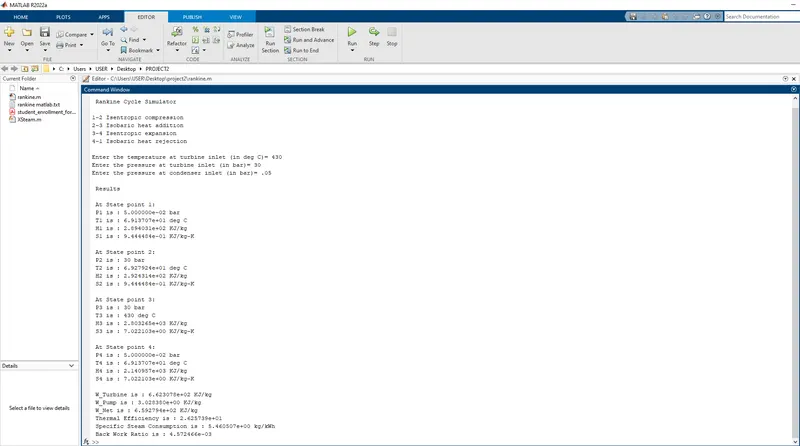
• First, we are displaying all the processes that happen during the rankine cycle working like isentropic compression, isobaric heat addition, isentropic expansion and isobaric heat rejection
• After that, we find out the values required for saturation curves and the values of critical point of water using linspace command for saturation temperature and preset values for critical temperature and pressure. Then the XSteam command is to find the saturation enthalpy & entropy and critical enthalpy & entropy.
• We find out the values of pressure, temperature, entropy and enthalpy across all the points in the rankine cycle like boiler, turbine, condenser and pump outlets using the XSteam command. Initially the values of turbine inlet temperature (T3) & pressure (P3) and condenser inlet pressure (P4) are provided as user defined inputs.
• Then, we find out the values of pressure, temperature, entropy and enthalpy across the subcooled liquid and superheated vapour regions using XSteam command and for loops for entropy in super subcooled liquid and superheated vapour regions.
• Then we find the Thermal Efficiency, Specific Steam Consumption and Back Work Ratio by calculating the values of work done by turbine, pump and heat input to the boiler.
• We then plot the graphs for all found saturation points and critical points between temperature & entropy and enthalpy & entropy and the title, labels are given for each of the plots.
• Finally we, print all the values of tempratures, pressures, entropies and enthalpies at the all state points and then the values of workdone by turbine, pump, net workdone, thermal efficiency, specific steam consumption and back work ratio are printed.

Outputs