Week 4.1 - Genetic Algorithm

WEEK 4.1: GENETIC ALGORITHM

AIM: To optimise and find the global maxima of stalagmite function using genetic algorithm in Matlab.

THEORY:
Concept of Genetic Algorithm
1) Genetic Algorithms are adaptive heuristic search algorithms that belong to the larger part of evolutionary algorithms. Genetic algorithms are based on the ideas of natural selection and genetics.
2) Genetic Algorithm is a search-based optimization technique based on the principles of Genetics and Natural Selection. It is frequently used to find optimal or near-optimal solutions to difficult problems which otherwise would take a lifetime to solve. It is frequently used to solve optimization problems, in research, and in machine learning.
3) The steps involved in genetic algorithm are as shown below in flow chart:

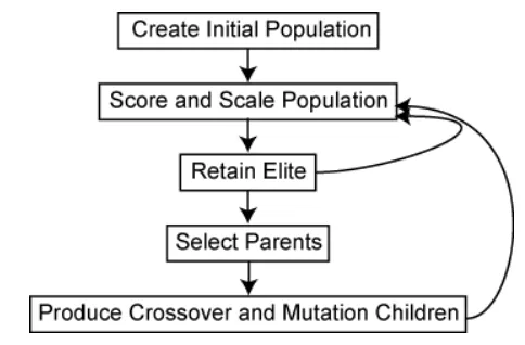
4) The genetic algorithm in short is;

1. Randomly initialize populations
2. Determine fitness of population
3. Until convergence repeat:
   a) Select parents from population
   b) Crossover and generate new population
   c) Perform mutation on new population
   d) Calculate fitness for new population

5)The genetic algorithm is thus used in many applications which can be related to financial markets, manufacturing processes, image processing, traffic management and in many other scenarios.

Stalagmite Function:
Stalagmite Function is a mathematical model which is used to determine the local minima and maxima. Its named after the rock formation that arises from floor in caves due to accumulation of materials that are deposited on the floor from ceiling drippings.

The stalagmite function is given as;
`f_(1,x)=[sin⁡(5.1πx+0.5)]^6`
`f_(1,y)=[sin⁡(5.1πy+0.5)]^6`
`f_(2,x)=exp⁡[-4ln⁡(2)(x-0.0667)^2/0.64]`
`f_(2,y)=exp⁡[-4ln⁡(2)(y-0.0667)^2/0.64]`
`:. f(x,y)=f_(1,x)×f_(1,y)×f_(2,x)×f_(2,y)`

PROCEDURE:
1) We first create a function to determine the stalgmite function.

function [f] = stalagmite(input_vector)
x= input_vector(1);
y= input_vector(2);
f1 = (sin(5.1*pi*x + 0.5)).^6;
f2 = exp(-4*log(2)*((x-0.0667).^2)./0.64);
f3 = (sin(5.1*pi*y + 0.5)).^6;
f4 = exp(-4*log(2)*((y-0.0667).^2)./0.64);
f = -(f1*f2*f3*f4);
end

2) Then to check whether the stalagmite gives the required output a code is written to verify whether a 3D plot is generated.

clear
close
clc

%Initial input Values 
low_b= input('Enter the Lower Bound Value: ');
up_b= input('Enter the Upper Bound Value: ');

% Input Variables with proper line spaces
x= linspace(low_b,up_b,150);
y= linspace(low_b,up_b,150);

% 3D Matrix creation
[xx, yy] = meshgrid(x,y);


count = 50;     % Giving the Count/ Number of Iterations for the optimal generation
%Stopwatch timer is used
tic            
for i = 1:length(xx)
    for j=1:length(yy)
        input_vector(1)= xx(i,j);
        input_vector(2)= yy(i,j);
        f(i,j)=stalagmite(input_vector);
    end
end

study_time = toc;  
figure(1)
surfc(xx,yy,-f)
shading interp
xlabel('x label')
ylabel('y label')
legend('X Values','Y values')
title('Stalagmite Function')
saveas(1, 'Stalagmite.png')
% [x, fval]= ga(@stalagmite,2)

3) For the first condition i.e the unbounded/ random sampling inputs the the code is as given below;

%Study 1 Unbounded/random sampling Inputs
tic

for i= 1:count
    [inputs,fopt(i)]= ga(@stalagmite,2);
    xopt(i)= inputs(1);
    yopt(i)= inputs(2);
end

studytime_1 =toc;

figure(2)
subplot(2,1,1)
surfc(x,y,-f)
shading interp
title('Unbounded Inputs')
xlabel('x value')
ylabel('y value')

hold on 
plot3(xopt,yopt,-fopt,'marker','o', 'markersize',5,'markerfacecolor','r');
subplot(2,1,2)
plot(-fopt)
xlabel('Iterations')
ylabel('Function Maximum')
saveas(2,'Unbound Inputs.png')

4) Then the code for the 2nd condition which is for bounded input is as shown below;

%Study 2 - Statistical Behaviour With upper and lower Bound sampling 
%(Bounded Inputs)
tic
for i = 1:count
    [inputs, fopt(i)]= ga(@stalagmite, 2, [],[],[],[], [low_b;low_b],[up_b;up_b]);
    xopt(i)= inputs(1);
    yopt(i)= inputs(2);
end
studytime_2 = toc;

figure(3)
subplot(2,1,1) 
surfc(x,y,-f)
shading interp
title('Bounded Inputs')
xlabel('x value')
ylabel('y value')

hold on

plot3(xopt,yopt,-fopt, 'marker','o', 'markersize', 5, 'markerfacecolor', 'm')
subplot(2,1,2)
plot(-fopt)
xlabel(' Iterations' )
ylabel('Function Maximum')
saveas(3, 'Bounded Input.png')

5) Then the code for the final condition which for bounded input with increasing the populationsize is;

%Study 3 - code for Upper and Lower bound sampling and increase the population size
options = optimoptions(@ga);
options = optimoptions(options,'populationsize',170);

tic;
for i=1:count
    [inputs,fopt(i)]= ga(@stalagmite,2,[],[],[],[],[low_b;low_b],[up_b;up_b],[],[],options);
    xopt(i)= inputs(1);
    yopt(i)= inputs(2);
end

studytime_3 = toc;
figure(4)
subplot(2,1,1)
surfc(x,y,-f)
shading interp
title('Bounded Inputs with modified population size')
xlabel('x value')
ylabel('y value')

hold on 

plot3(xopt,yopt,-fopt, 'marker','o','markersize',5,'markerfacecolor','c')
subplot(2,1,2)
plot(-fopt)
xlabel('Iterations')
ylabel('Function Maxima')
saveas(4, 'Bounded Inputs with modified population size.png')

global_maxima = -fopt;      % Finding the Global Maxima

Explanation of ga function:

"ga' is an inbuilt Matlab function which is used for genetic algorithm to find the global minima.

Syntax for “ga ()” command is as follows:

• X = ga(fun,nvars) find the local unconstrained minimum x , to the objective function (fun); and nvars is the dimension (no. of design variable) of fun.
• X = ga(fun,nvars,A,b,Aeq,beq,lb,ub) defines the set of lower and upper bounds on the design variables x, so that the solution is found in the range ub,{ Set A = [] and b = [] if no linear inequalities exist } . { Set Aeq = [] and beq = [] if no linear equalities exist.}
• x = ga(fun,nvars,A,b,Aeq,beq,lb,ub,nonlcon,options) minimizes with the default optimization parameters replaced by values in options. (Set nonlcon=[] if no nonlinear constraints exist.) Create options using optimoptions.

‘ga ()’ always calculates the value for ‘x’ where the function is minimum ,thus gives us the global minima.But we need to calculate global maxima in our code ,So to achieve that we are minimizing the fitting function with a “ – “ (minus) symbol, because Maximizing f(x,y) is the same as minimizing –f(x,y).
That is the reason we have put” – “ (minus) symbol in the equation of “fopt” in the function code.

OUTPUT:

1) For the first condition i.e the unbounded/ random sampling inputs the the output graph is as given below: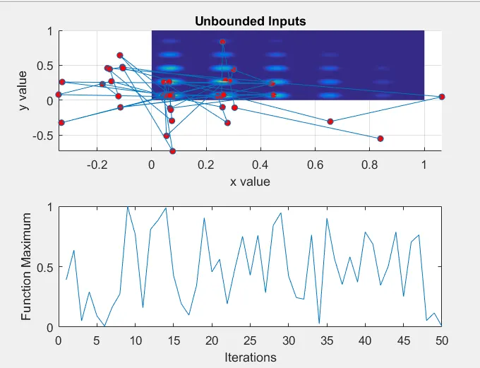

2) For the 2nd condition which is for bounded input, the output graph is as shown below: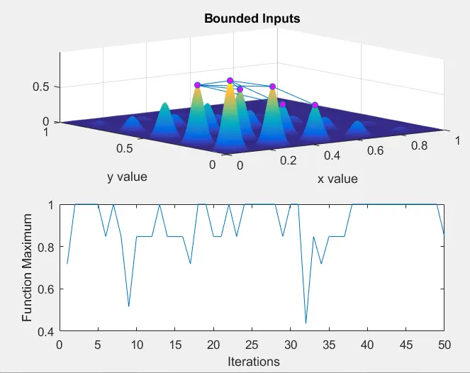

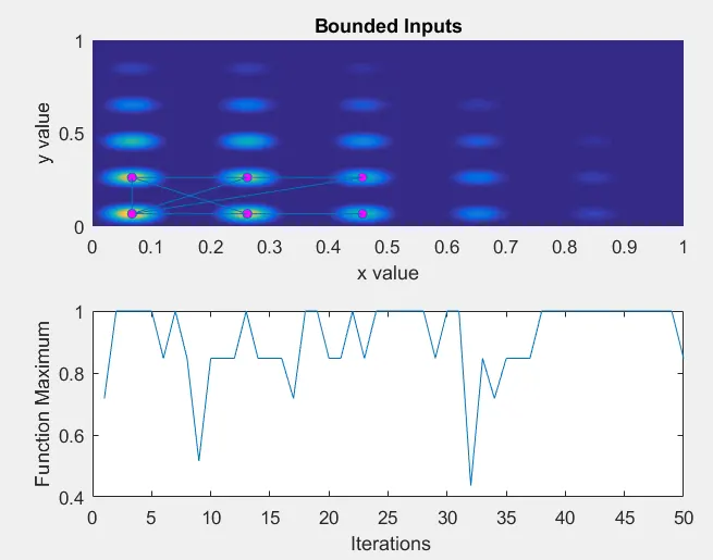
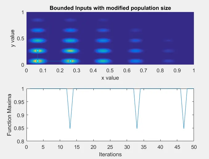
3) For the 3rd condition for which bounded input with increasing the populationsize, the output is: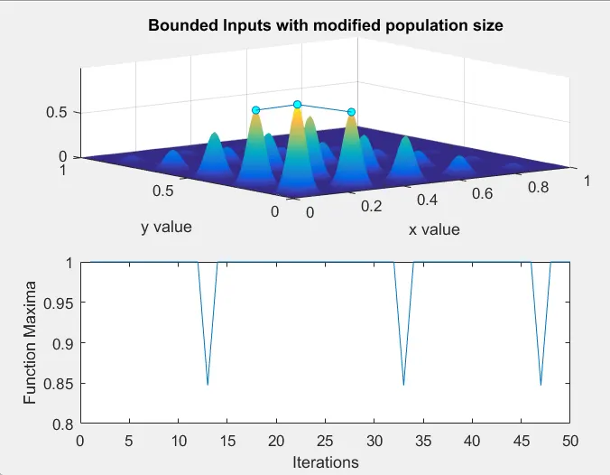

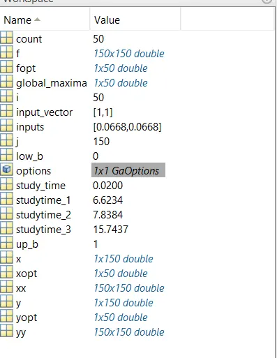
Workspace Output:

CONCLUSION:

1) When 'ga' is unbounded it tries to find the solution outside the given limits. The accuracy is also low as we can observe that the function maxima vs iteration graph has found the maxima only twice.

2) For bounded inputs the accuracy is better than the unbounded condition ga as its bounded to the workspace but requires a little bit more time to find the maxima.

3) For bounded inputs with modified population, the ga function tries to find global maxima in the specific population that is defined. So its highly accurate method to find the global maxima but takes more time compared to other two conditions.

LEARNING OUTCOME:

• Learnt what is genetic algorithm and its application\
• How to find the global minima and maxima using ga function in matlab