Project 2 - Rankine cycle Simulator
Rankine Cycle Simulator
AIM: To create a Rankine Cycle Simulator using MATLAB.
OBJECTIVES:
1. To calculate the state points of the Rankine Cycle.
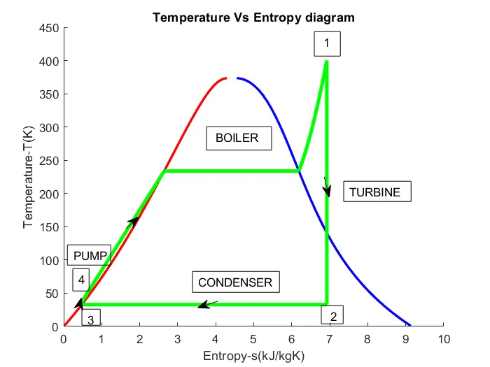
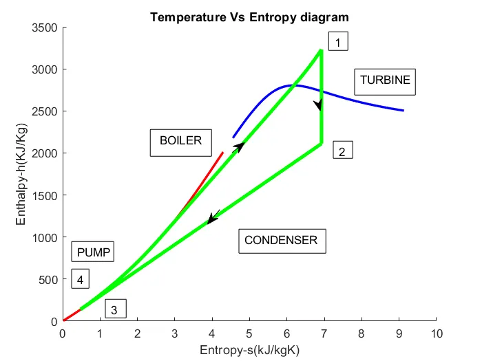
2. To plot the corresponding T-s and h-s plots for the given set of inputs.
3. To calculate
- Net work output
- Back work ratio
THEORY:
The Rankine cycle is an idealized thermodynamic cycle describing the process by which certain heat engines, such as steam turbines or reciprocating steam engines, allow mechanical work to be extracted from a fluid as it moves between a heat source and heat sink. The Rankine cycle is named after William John Macquorn Rankine, a Scottish polymath professor at Glasgow University.
For each process in the vapour power cycle., it is possible to assume a hypothetical or ideal process that represents the basic intended operation and involves no extraneous effects. For the steam boiler, this would be a reversible constant pressure heating process of water to form steam, for the turbine the ideal process would be a reversible adiabatic expansion of steam, for the condenser it would be a reversible constant pressure heat rejection as the steam condenses till it becomes saturated liquid, and for the pump, the ideal process would be the reversible adiabatic compression of this liquid ending at the initial pressure. When all these four processes are ideal, the cycle is an ideal cycle, called a Rankine cycle. This
is a reversible cycle.
The cycle has been plotted on the p-v, T-s, and h-s planes. The numbers on the plots correspond to the numbers on the flow diagram. For any given pressure, the steam approaching the turbine may be dry saturated (state1) wet (state 1 '), or superheated (state l"), but the fluid approaching the pump is, in each case, saturated liquid (State 3). Steam expands reversibly and adiabatically in the turbine from state 1 to state 2 (or1' to 2', or 1" to 2"), the steam leaving the turbine condenses to water in the condenser reversibly at constant pressure from state 2 (or 2', or 2") to state 3, the water at state 3 is then pumped to the boiler at state 4 reversibly and adiabatically, and the water is heated in the boiler to form steam reversibly at constant pressure from state 4 to state 1 (or 1' or1").
1-2 isentropic expansion in the Turbine
2-3 const pr heat rejection by the Condenser
3-4 isentropic compression in the Pump
4-1 const pr heat addition by the Boiler
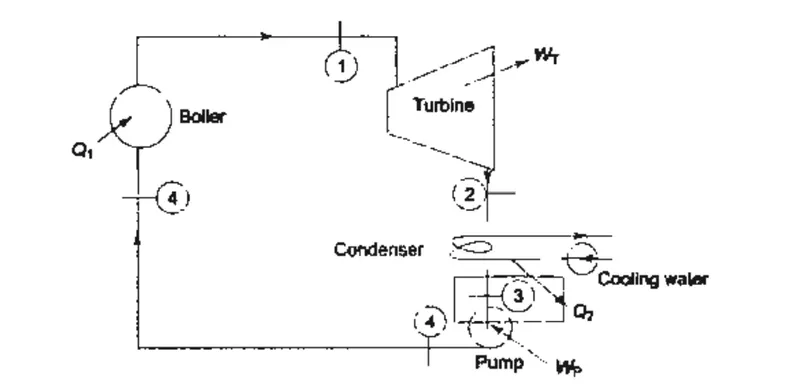
A simple steam power plant
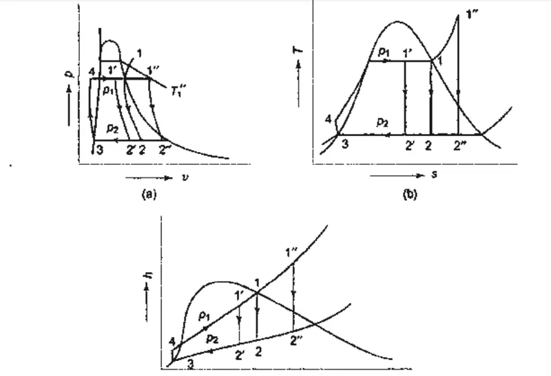
Rankine cycle p-v, T-s, and h-s diagram
Rankine cycle
Given Inputs:
- Turbine Inlet temperature = 400° C
- Turbine Inlet Pressure = 30 bars
- Turbine Outlet Pressure = 0.05 bars = Condenser Inlet Pressure
Xsteam library :https://drive.google.com/file/d/1RK_fvrOj38CIaQvmLT1S3daqHnxKCGU-/view
PROGRAMMING:
clear all
close all
clc

% Programme to create Rankine cycle simulation

%Thermodynamic processes
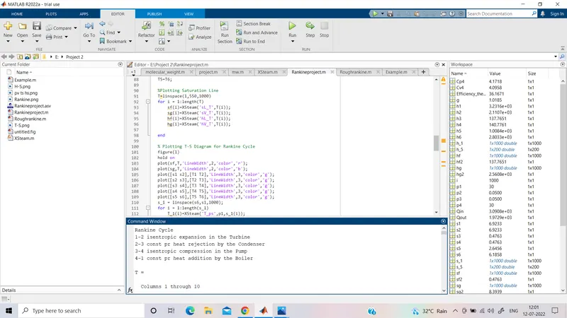
fprintf('Rankine Cycle\n');
fprintf('1-2 isentropic expansion in the Turbine\n');
fprintf('2-3 const pr heat rejection by the Condenser\n');
fprintf('3-4 isentropic compression in the Pump\n');
fprintf('4-1 const pr heat addition by the Boiler\n');

% Inputting pressure and temperature(given)
p1=30; %the pressure at Turbine inlet in bar
T1=400; %the temperature at Turbine inlet in degree celcius
p2=0.05; %the pressure at Condenser inlet in bar

% Calculating state variable from given data file at point 1
h1=XSteam('h_pT',p1,T1);
s1=XSteam('s_pT',p1,T1);

% Calculating state variable from given data file at point 2
s2=s1;
sg2=XSteam('sV_p',p2);
sf2=XSteam('sL_p',p2);
x2=(s1-sf2)/(sg2-sf2);
s1=sf2+x2*(sg2-sf2);
hf2=XSteam('hL_p',p2);
hg2=XSteam('hV_p',p2);
h2=hf2+x2*(hg2-hf2);

% Calculating state variable from given data file at point 3
p3=p2;
s3=XSteam('sL_p',p3);
h3=XSteam('hL_p',p3);
T3=XSteam('Tsat_p',p3);

% Calculating state variable from given data file at point 4
s4=s3;
p4=p1;

% Calculating temperature,T4
Cp4 = XSteam('Cp_ps',p4,s4);
Cv4 = XSteam('Cv_ps',p4,s4);
g=Cp4/Cv4;
w=(g-1)/g;
T4=T3*((p4/p3)^w);


% Calculating temperature, T2
T2=T3;

%Turbine work
W_T=h1-h2;

%Pump work
v3=XSteam('VL_p',p3);
W_p=v3*(p4-p3)*100;
h4=W_p+h3;


% Net work (Rankine Cycle)
W_net = W_T - W_p;

%heat addition by the Boiler
Qin=h1-h4;

%heat rejection by the Condenser
Qout=h2-h3;

%Thermal Efficiency of Rankine Cycle
Efficiency_thermal=(W_net/Qin)*100;

%specific steam consumption
SSC=3600/W_net;

%back_work_ratio
% WR= W_p/ W_T;

%Calculation  of  T5,T6,s5,s6,h5,h6
T6=XSteam ('Tsat_p', p1) ;
s5=XSteam ('sL_p', p1) ;
s6=XSteam ('sV_p', p1) ;
h5=XSteam ('hL_p', p1) ;
h6=XSteam ('hV_p', p1) ;
T5=T6;

%Plotting Saturation Line
T=linspace(1,550,1000)
for i = 1:length(T)
    sf(i)=XSteam('sL_T',T(i));
    sg(i)=XSteam('sV_T',T(i));
    hf(i)=XSteam('hL_T',T(i));
    hg(i)=XSteam('hV_T',T(i));

end

% Plotting T-S Diagram for Rankine Cycle
figure(1)
hold on
plot(sf,T,'LineWidth',2,'color','r');
plot(sg,T,'LineWidth',2,'color','b');
plot([s1 s2],[T1 T2],'LineWidth',3,'color','g');
plot([s2 s3],[T2 T3],'LineWidth',3,'color','g');
plot([s3 s4],[T3 T4],'LineWidth',3,'color','g');
plot([s4 s5],[T4 T5],'LineWidth',3,'color','g');
plot([s5 s6],[T5 T6],'LineWidth',3,'color','g');
s_1 = linspace(s6,s1,1000);
for i = 1:length(s_1)
    T_1(i)=XSteam('T_ps',p1,s_1(i));
end
plot(s_1,T_1,'LineWidth',3,'color','g');
xlabel('Entropy-s(kJ/kgK)');
ylabel('Temperature-T(K)');
title ('Temperature Vs Entropy diagram')

% Plotting H-S Diagram for Rankine Cycle
figure(2)
hold on
plot(sf,hf,'LineWidth',2,'color','r');
plot(sg,hg,'LineWidth',2,'color','b');
plot([s1 s2],[h1 h2],'LineWidth',3,'color','g');
plot([s2 s3],[h2 h3],'LineWidth',3,'color','g');
plot([s3 s4],[h3 h4],'LineWidth',3,'color','g');
h_5 = linspace(h4,h5,200);
for i = 1:length(h_5)
    s_5(i)=XSteam('S_ph',p1,h_5(i));
end
plot(s_5,h_5,'LineWidth',3,'color','g');
plot([s5 s6],[h5 h6],'LineWidth',3,'color','g');
s_1 = linspace(s6,s1,1000);
for i = 1:length(s_1)
    h_1(i)=XSteam('h_ps',p1,s_1(i));
end
plot(s_1,h_1,'LineWidth',3,'color','g');
xlabel('Entropy-s(kJ/kgK)');
ylabel('Enthalpy-h(KJ/Kg)');
title ('Temperature Vs Entropy diagram')

%dispalying output
fprintf('At state point 1\n');
fprintf('P1 % .2f Bar\n',p1);
fprintf('T1 % .2f degree celcius\n',T1);
fprintf('h1 % .2f KJ/Kg\n',h1);
fprintf('s1 % .2f kJ/kgK\n',s1);

fprintf('At state point 2\n');
fprintf('P2 % .2f Bar\n',p2);
fprintf('T2 % .2f degree celcius\n',T2);
fprintf('h2 % .2f KJ/Kg\n',h2);
fprintf('s2 % .2f kJ/kgK\n',s2);
fprintf('x2 %.2f \n',x2);

fprintf('At state point 3\n')
fprintf('P3 % .2f Bar\n',p3);
fprintf('T3 % .2f degree celcius\n',T3);
fprintf('h3 % .2f KJ/Kg\n',h3);
fprintf('s3 % .2f kJ/kgK\n',s3);

fprintf('At state point 4\n')
fprintf('P4 % .2f Bar\n',p4);
fprintf('T4 % .2f degree celcius\n',T4);
fprintf('h4 % .2f KJ/Kg\n',h4);
fprintf('s4 % .2f kJ/kgK\n',s4);

fprintf('Turbine work % .2f KJ/Kg\n',W_T)
fprintf('Pump work % .2f KJ/Kg\n',W_p)
fprintf('net work % .2f KJ/Kg\n',W_T - W_p)
fprintf('Thermal efficiency of Rankine Cycle  % .2f percent\n',(W_net/Qin)*100)
fprintf('Specific steam consumpition  % .2f Kg/KWh\n',3600/W_net)
fprintf('back_work_ratio %.3f \n',W_p/ W_T)
OUTPUTS:
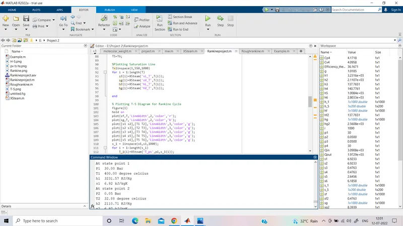
At state point 1
P1 30.00 Bar
T1 400.00 degree celcius
h1 3231.57 KJ/Kg
s1 6.92 kJ/kg K
At state point 2
P2 0.05 Bar
T2 32.88 degree celcius
h2 2110.71 KJ/Kg
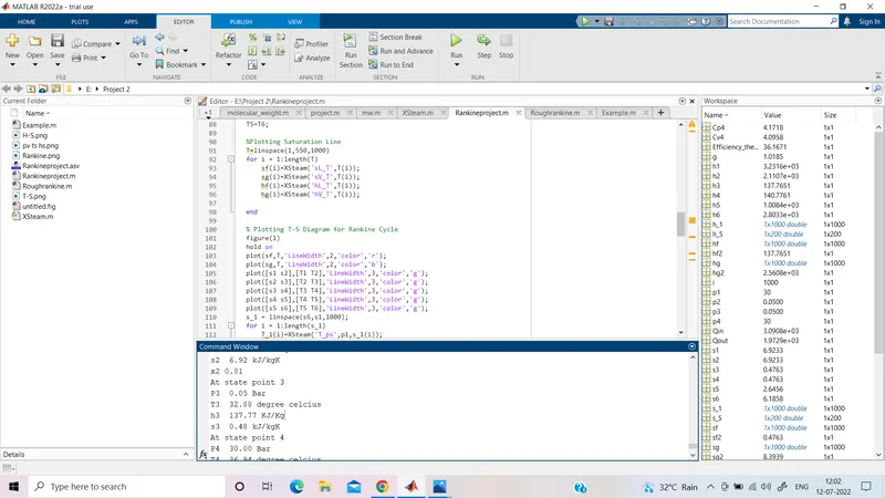
s2 6.92 kJ/kg K
x2 0.81
At state point 3
P3 0.05 Bar
T3 32.88 degree celcius
h3 137.77 KJ/Kg
s3 0.48 kJ/kg K
At state point 4
P4 30.00 Bar
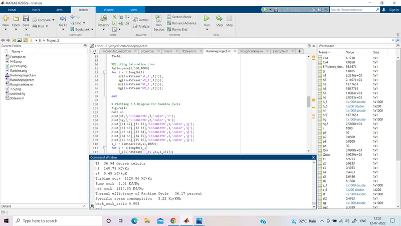
T4 36.94 degree celcius
h4 140.78 KJ/Kg
s4 0.48 kJ/kg K
Turbine work 1120.86 KJ/Kg
Pump work 3.01 KJ/Kg
net work 1117.85 KJ/Kg
Thermal efficiency of Rankine Cycle 36.17 percent
Specific steam consumption 3.22 Kg/KWh
back_work_ratio 0.003
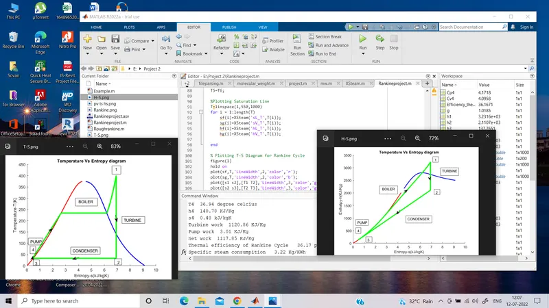
PROCEDURE:
Step1:clear all, close all, clc used to clear any previously defined values.
Step2:A suitable programme name is given.
Step3:Display 4 processes in the command window by 'fprintf()' command.
Step4:Given data are inputted.
Step5:Using the given inputs all four stage points are calculated by XSteam command.
(H-Enthalpy, S-Entropy, T-Temperature, P-Pressure, x-Dryness factor, )
Step6:After calculating all parameters, the Pump work, Turbine Work, Net work output, Back Work Ratio, specific steam consumption, and Thermal Efficiency are calculated.
Step7:To plot the graph, h-S & T-s, plot command, and for loop command are used.
Step8: To display all output 'fprintf()' command is used.
ERROR: No such major error is found.
CONCLUSION: Rankine cycle simulation successfully performed.
REFERENCES:
https://en.wikipedia.org/wiki/Rankine_cycle
https://www.learnthermo.com/T1-tutorial/ch09/lesson-E/pg10.php
Basic and Applied Thermodynamics - P.K Nag