Week 4.1 - Genetic Algorithm

Aim: To understand the concept of Genetic Algorithm (GA) with an optimisation of Mathematical Stalagmite function .

• To write a code in MATLAB to optimise the stalagmite function and find the global maxima of the function.
• To expalin the concept of genetic algorithm in simple words and also explain the syntax for Genetic Algorithm in MATLAB.
• To ensure that the code gives the same output, even if it is made to run several times.
• To Plot graphs for all studies and for stalagmite function maximum vs no. of iterations.

Theory:

Genetic Algorithm (GA):

Genetic algorithm is a population-based probabilistic search and optimization techniques, which works based on the mechanisms of natural selection and natural genetics. It simulates the process of Evolution.

It is ased on the Survival of the fittest concept given by Charles Darwin.

Genetic Algorithm(GA) first developed by Prof. John Holland (1975) at the University of Michigan. Evolution is the optimisation process, is the key idea behind the developement of Genetic Algorithms (GA). The Robustness that is balance between efficiency and efficacy is necessary for the survival in the many different environment conditions, is the central theme under the developement of genetic algorithms (GA).

GA is an iterative searching technique usually works in cycles with or without convergence criteria. Solution is not neccessarily gauranteed as it can end with local optima due to random selection procedure, but modified selection techniques increase the solution accuracy.

Work flow of Genetic Algorithm(GA):

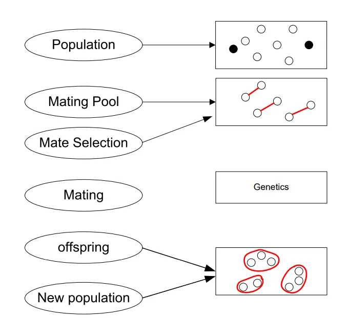
Biological Evolution Process		Mimicked Genetic Algorithm Flow chart

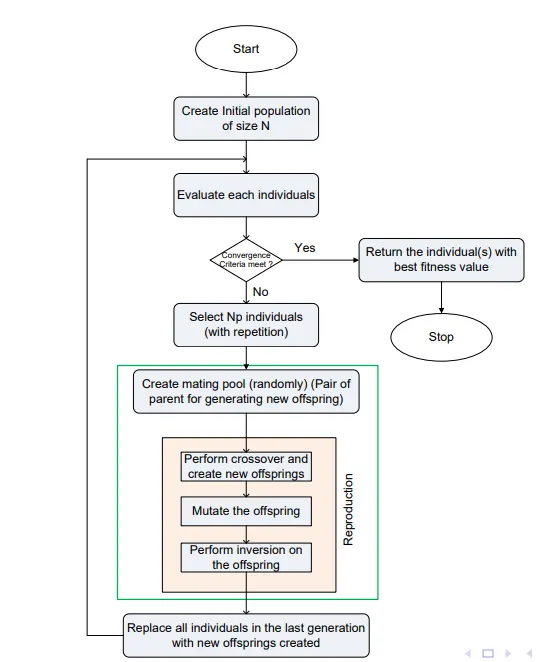• Initially population of trial solutions is selected with `2n` to `4n` is selected where `n`is number of variables.
• Each solution is usually represented by string of variables either binary or encoded. These correspond to the chromosomes in the genetics.
• The string length can be made large enough to achieve any desired fitness of approximation and thus any desired accuracy can be achieved.
• This is how mating pool is made and selection of mating partner is done and offsprings are produced by crossover of mating partners (Parents).
• These offsprings represent the new generation of solutions. These are also checked with fittness function criteria and
  only best are selected for next mating pool by discarding the unfit. Survival of the fittest!
• Some changes are introduced randomly in to the offsprings if needed to mimic mutation. These may be advantageous or disadvantageous.
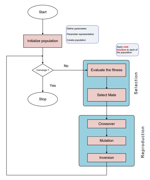
• Then old population is then replaced with new genartion and the process of crossover, fittness evaluation, selection of the best and
  mutation(if desired) is repated till the convergence criteria is achieved.
• The final optimised solution is given as output.

Derrived Flowchart for Genetic Algorithm(GA):

Salient features of GA:

• It does not require any derivative information (which may not be available for many real-world problems).
• It has overlapping generation (Only fraction of individuals are replaced).
• It is faster and more efficient as compared to the traditional methods.
• It is computationally expensive as fitness evaluation is done repeatatively.
• It has very good parallel capabilities.
• It optimizes both continuous and discrete functions and also multi-objective problems.
• Useful when the search space is very large and there are a large number of parameters involved.
• It is better to use when initial population size is large.
• It always gets an answer to the problem, which gets better over the time.
• It provides a list of good solutions not a single solution.
• Selection is biased toward more highly fit individuals; Hence, the average fitness (of overall population) is expected to increase insuccession.
• The best individual may appear in any iteration.

Syntax for Genetic Algorithm (GA) in MATLAB:

1. Syntax for passing the inputs:
   • x = ga(fun,nvars) which finds a local unconstrained minimum, x, to the objective function, fun. nvars is the dimension (number of design variables) of fun.
   • x = ga(fun,nvars,A,b) which finds a local minimum x to fun, subject to the linear inequalities A*x ≤ b. ga evaluates the matrix product A*x as if x is transposed (A*x').
   • x = ga(fun,nvars,A,b,Aeq,beq) which finds a local minimum x to fun, subject to the linear equalities Aeq*x = beq and A*x ≤ b. (Set A=[] and b=[] if no linear inequalities exist.) ga evaluates the matrix product Aeq*x as if x is transposed (Aeq*x').
   • x = ga(fun,nvars,A,b,Aeq,beq,lb,ub) which defines a set of lower and upper bounds on the design variables, x, so that a solution is found in the range lb ≤ x ≤ ub. (Set Aeq=[] and beq=[] if no linear equalities exist.)
   • x = ga(fun,nvars,A,b,Aeq,beq,lb,ub,nonlcon) which subjects the minimization to the constraints defined in nonlcon. The function nonlcon accepts x and returns vectors C and Ceq, representing the nonlinear inequalities and equalities respectively. ga minimizes the fun such that C(x) ≤ 0 and Ceq(x) = 0. (Set lb=[] and ub=[] if no bounds exist.)
   • x = ga(fun,nvars,A,b,Aeq,beq,lb,ub,nonlcon,options) which minimizes with the default optimization parameters replaced by values in options. (Set nonlcon=[] if no nonlinear constraints exist.) Create options using optimoptions.
   • x = ga(fun,nvars,A,b,Aeq,beq,lb,ub,nonlcon,intcon) or
     x = ga(fun,nvars,A,b,Aeq,beq,lb,ub,nonlcon,intcon,options) requires that the variables listed in intcon take integer values.
     
     
     
2. Syntax for required output parameters:
   • x = ga(problem) finds the minimum for problem, a structure described above for passing inputs.
   • [x,fval] = ga(___), for any previous input arguments, also returns fval, the value of the fitness function at x.
   • [x,fval,exitflag,output] = ga(___) also returns exitflag, an integer identifying the reason the algorithm terminated, and output, a structure that contains output from each generation and other information about the performance of the algorithm.
   • [x,fval,exitflag,output,population,scores] = ga(___) also returns a matrix population, whose rows are the final population, and a vector scores, the scores of the final population.

MATLAB code to optimise mathematical Stalagmite function for global maxima:

In this code stalagmite function is modified to obtain global maxima as GA gives global minima. It has been seen into the code for stalagmite function where output of function has been multiplied by -1. (The substraction of output of function from 1 will also work out).

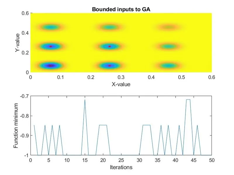
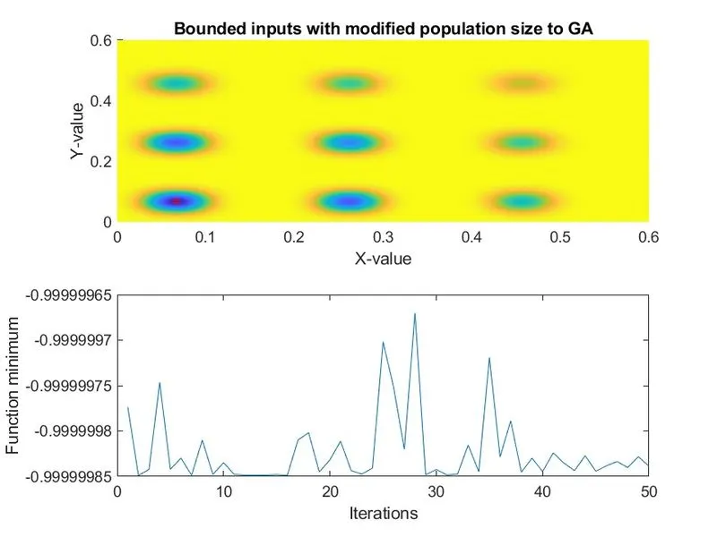
The statistical behavoiur has been studied for three cases as follows:

1) With unbounded inputs to GA.

2) With bounded inputs to GA.

3) With bounded inputs and modified population size to GA.

The results of the same have been represented here.

MATLAB Code:

% Optimisation of Stalagmite function using genetic algorithm
close all;
clear all;
clc;

% Defining search space
x=linspace(0,0.6,150);
y=linspace(0,0.6,150);
num_cases=50;              % Initialisation of Number of iteration of GA

% Creating a 2D mesh
[xx,yy] = meshgrid(x,y);

% Evaluationg the Stalagmite Function over meshgrid
for i=1:length(xx)
    for j=1:length(yy)
        input_vector(1)=xx(i,j);
        input_vector(2)=yy(i,j);
        f(i,j)=stalagmite_max(input_vector);
    end
end


%% Study 1 -Statistical behaviour
tic
for i=1:num_cases
   [inputs,fval]= ga(@stalagmite_max,2);
   xopt(i)= inputs(1);
   yopt(i)= inputs(2);
   fopt(i)= fval;
end
study1_time = toc;              % Measuring time elapsed in calculation over number of ga iterations

%Plotting the results
figure(1)
subplot(2,1,1)
hold on
surfc(x,y,f);
shading interp;
plot3(xopt,yopt,fopt,'Marker','o','MarkerSize',5,'MarkerFaceColor','r');
title('Unbounded inputs to GA');
xlabel('X-value');
ylabel('Y-value');
subplot(2,1,2)
plot(fopt);
xlabel('Iterations');
ylabel('Function minimum');
saveas(gcf,'Unbounded inputs to GA','jpg');

%% Study 2 -Statistical behaviour - with upper and lower bounds
tic
for i=1:num_cases
   [inputs,fval]= ga(@stalagmite_max,2,[],[],[],[],[0,0],[0.6,0.6]);
   xopt(i)= inputs(1);
   yopt(i)= inputs(2);
   fopt(i)= fval;
end
study2_time = toc;         % Measuring time elapsed in calculation over number of ga iterations

%Plotting the results
figure(2)
subplot(2,1,1)
hold on
surfc(x,y,f);
shading interp;
plot3(xopt,yopt,fopt,'Marker','o','MarkerSize',5,'MarkerFaceColor','r');
title('Bounded inputs to GA');
xlabel('X-value');
ylabel('Y-value');
subplot(2,1,2)
plot(fopt);
xlabel('Iterations');
ylabel('Function minimum');
saveas(gcf,'Bounded inputs to GA','jpg');

%% Study 3 -Statistical behaviour - with upper and lower bounds
options = optimoptions('ga');
options = optimoptions(options,'PopulationSize',170);      % Defining input-options with optimoptions

tic
for i=1:num_cases
   [inputs,fval]= ga(@stalagmite_max,2,[],[],[],[],[0,0],[0.6,0.6],[],[],options);
   xopt(i)= inputs(1);
   yopt(i)= inputs(2);
   fopt(i)= fval;
end
study3_time = toc;            % Measuring time elapsed in calculation over number of ga iterations

%Plotting the results
figure(3)
subplot(2,1,1)
hold on
surfc(x,y,f);
shading interp;
plot3(xopt,yopt,fopt,'Marker','o','MarkerSize',5,'MarkerFaceColor','r');
title('Bounded inputs with modified population size to GA');
xlabel('X-value');
ylabel('Y-value');
subplot(2,1,2)
plot(fopt);
xlabel('Iterations');
ylabel('Function minimum');
saveas(gcf,'Bounded inputs with modified population size to GA','jpg');

Function Code: stalagmite_max.m

function [fs] = stalagmite_max(v)
x = v(1);                           % X part of input vector
y = v(2);                           % Y part of input vector
f1x = (sin((5.1*pi*x)+0.5))^6;               % F1x of stalagmite function
f1y = (sin((5.1*pi*y)+0.5))^6;               % F1y of stalagmite function
f2x = exp((-4*log(2)*(x-0.0667)^2/0.64)^1);  % F2x of stalagmite function
f2y = exp((-4*log(2)*(y-0.0667)^2/0.64)^1);  % F2y of stalagmite function

fs = -1*(f1x*f2x*f1y*f2y);                   % Stalagmite function   
                                     % Here modified by multiplying -1.      
end

The Results:

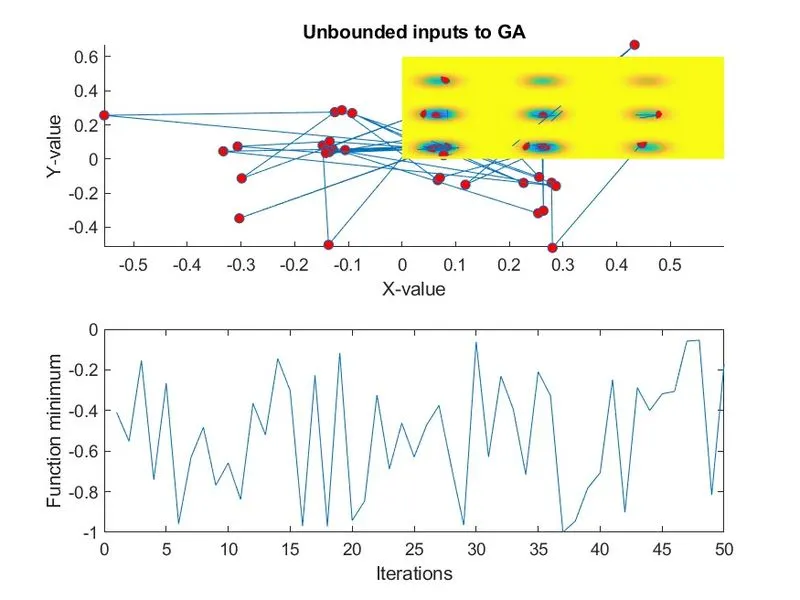
1) With unbounded inputs to GA:

2) With bounded inputs to GA:

3) With bounded inputs and modified population size to GA:

Observations and Conclusions:

1. The results with unbounded inputs show that the optimimum value varies with iteration as inputs are not bounded thus GA selecting individuals or samples from outside of the region of interest.
2. To minimise the randomness of the output we bounded the inputs to the GA into second case. The results show that the output is now constrained to the narrow band of the -0.7 to -1. Though it is varying in this band but it has been confined to this range as we gave lower and upper bounds. This highlights the impotance of knowing the lower and upper bounds of the solution for optimasation.
3. In the third case with bounded inputs we increased initial population size to 170 through the input options. This drastically improved the output by restricting it to the very very narrow range near to -1.
4. Thus it is clear that with lower and upper bounds of the solution samples the initial population size also plays very important role in the optimisation with the genetic algorithm (GA).