Week 4.1 - Genetic Algorithm
OBJECTIVE:
- To write a code in Matlab to optimize the stalagmite function and to find the global maxima of the function.
- Clearly explain the concept of genitic alogoritham in your words and explain the syntax of ga in Matlab
- Plot graphs for all 3 studies for Fmaximum vs no.of iteratios.
DEFINATION:
A genetic algorithm (GA) is a method for solving both constrained and unconstrained optimization problems based on a natural selection process that mimics biological evolution. The algorithm repeatedly modifies a population of individual solutions. At each step, the genetic algorithm randomly selects individuals from the current population and uses them as parents to produce the children for the next generation. Over successive generations, the population "evolves" toward an optimal solution.
Benfits of Optimization:
- Findin better design
- Faster design Evaluation
- Useful for trade - off analysis
- Non inteative design
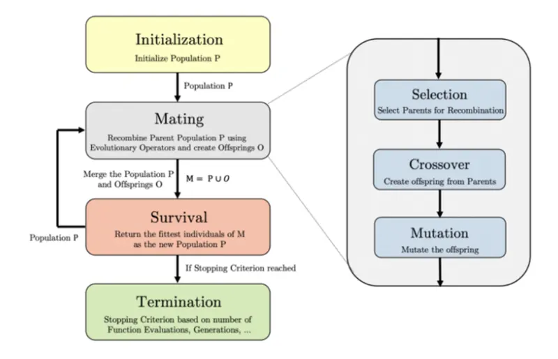
The above fig will explains about how the processor will work and what are the steps involved in g syntax.
PROCEDURE:
- Intially stalagmite function is defined ina seperate script
- A neggative sign is used in front of the function to obtain maxima of the function
- A nested for loop is utilized to iterate each of the element
- GA is used to determine the optimal of the function
- Plot is generated for different cases
The three cases consider are:
- Unbounded inputs
- Bounded inputs restricted with upper and lower bounds
- Bounded inputs with operations - increasing no of iterations by giving population size
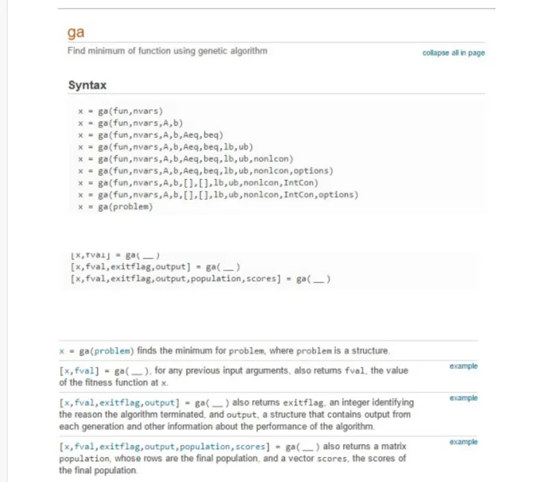
SYNTAX:
STALAGMITE FUNCTION:
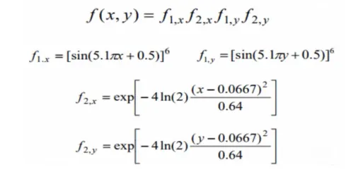
For the above function the stalagmite function code is fallows
Case:1 Using stalagmite model
Description of the function program: Intially function named as stalagmite is decleared that asscepts inputs_vector and returns an out put by calculating the f_1x, f_1y, f_2x and f_2y.
function [f] = stalagmite(input_vector)
x=input_vector(1);
y=input_vector(2);
f_1x=(sin(5.1*pi*x+0.5)).^6;
f_1y=(sin(5.1*pi*y+0.5)).^6;
f_2x=exp(-.4*log(2)*((x-0.0667).^2)./0.64):
f_2y=exp(-.4*log(2)*((y-0.0667).^2)./0.64):
f=-(f_1x.*f_2x.*f_1y.*f_2y);
end
Program Description:
Step1: firstly clear the command window and editor window by clear all close all clc
Step2:Linespace command is used to generate linear spaced vector by generating 150 points and spacing between the ponts is (0.6/0)/(150/1) which returns values for x and y variables.
Step3:Meshgrid will create 2D and 3D grids.The below command will return 2-D grid coordinates based in the coordinates contained in vectors x and y.
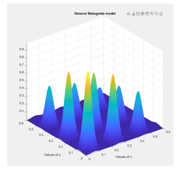
Step4:Evaluating the stalagmite function and plotting the fig with surface plot command.Below surface plate command will create a 3 Dimensional surfeace plot , which is a 3 dimensional surface that has solid edge colors and solid face colors.
clear all
close all
clc

% Defining our search space or one dimensional
x = linspace(0,0.6,150)
y = linspace(0,0.6,150)

% Creating a 2 Dimensional mesh
[xx,yy]=meshgrid(x,y)

% Evaluating the stalagmite function
for i=1:length(xx)
    for j = 1:length(yy)
        input_vector(1)=xx(i,j);
        input_vector(2)=yy(i,j);
        f(i,j)=stalagmite(input_vector);
    end
end
figure(1)
surfac(xx,yy,-f)%to create surface plot
shading interp %controls shading of surface and patch graphics objects
[inputs, favl]=ga(@stalagmite,2)
xlabel('values of x') %x-axis label
ylabel('values of y') %y-axis label
tittle('General stalagite moodel')
Out put: Global Maxiama
Case 2: Study without Boundtion:
Function get Stalagmite
clear all
close all
clc
% Defining our search space or one dimensional
x = linspace(0,0.6,150)
y = linspace(0,0.6,150)
% Giving number of iterations
[xx,yy]=meshgrid(x,y)
num_cases=50; value of iterations
f = get_stalagmite(x,y) %to generate the stalagmite function
tic %Calculating study time
% Evaluating the stalagmite function
for i=1: num_cases
[inputs, fopt(i)]=ga(@stalagmite,2) %storing
xopt(i)=inputs(1);
ypot(j)=inputs(2);
end
Study1_time=toc %to display the time taken
%Plotting
figure(1)
subplot(2,1,1) %to have multiple plots
surfc(x,y,-f)
hold on
shading interp
plot3(xpot,ypot,-fopt,'marker,'o','MarkerSize','5','MarkerFaceColor','r');
xlabel('values of x') %giving x axis label
ylabel('values of y') %giving y axis label
title('unbonded inputs')
subplot(2,1,2)
plot(-fpot);
xlabel('iterations')
ylabel('function min value')
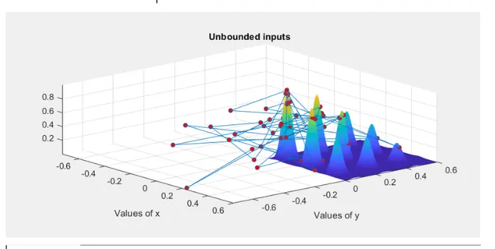
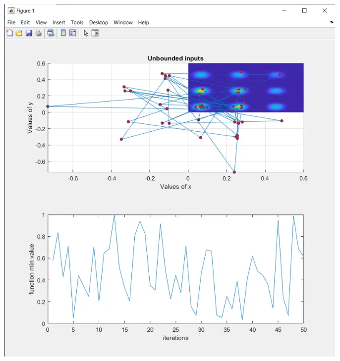
clear all
close all
clc

% Defining our search space or one dimensional
x = linspace(0,0.6,150)
y = linspace(0,0.6,150)

% Giving number of iterations
[xx,yy]=meshgrid(x,y)
num_cases=50; value of iterations
f = get_stalagmite(x,y) %to generate the stalagmite function
tic %Calculating study time
% Evaluating the stalagmite function
for i=1: num_cases
    [inputs, fopt(i)]=ga(@stalagmite,2,[],[],[],[],[0;0],[1;1]) %storing
    xopt(i)=inputs(1);
    ypot(j)=inputs(2);
end
Study1_time=toc %to display the time taken

%Plotting
figure(1)
subplot(2,1,1) %to have multiple plots
surfc(x,y,-f)
hold on
shading interp
plot3(xpot,ypot,-fopt,'marker,'o','MarkerSize','5','MarkerFaceColor','r');
xlabel('values of x') %giving x axis label
ylabel('values of y') %giving y axis label
title('Bonded inputs')
subplot(2,1,2)
plot(-fpot);
xlabel('iterations')
ylabel('function min value')OUTPUTS:
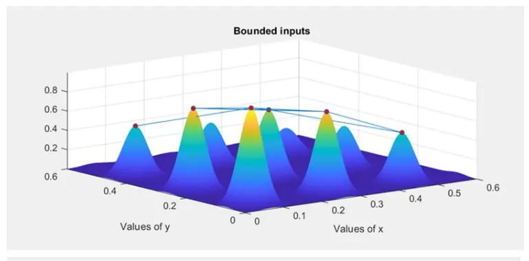
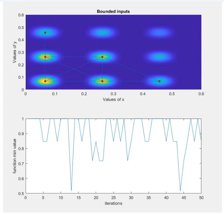
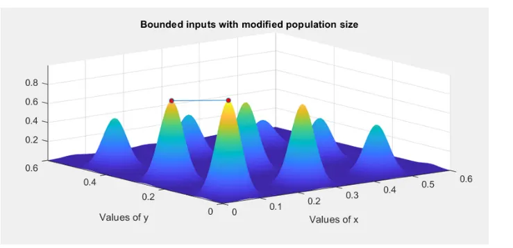
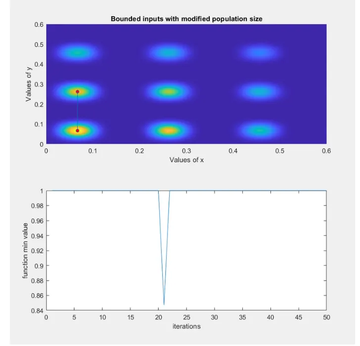
Case4:Study with modified poppulation size
Refer the below program incluuded in population size 400.The only change made is with below command.
Optioons=Optimooptions(Options,'Polution size',200)
In this study, the optimoptions command was used to increase the size of the population.
This method can be used for better fittness of the function
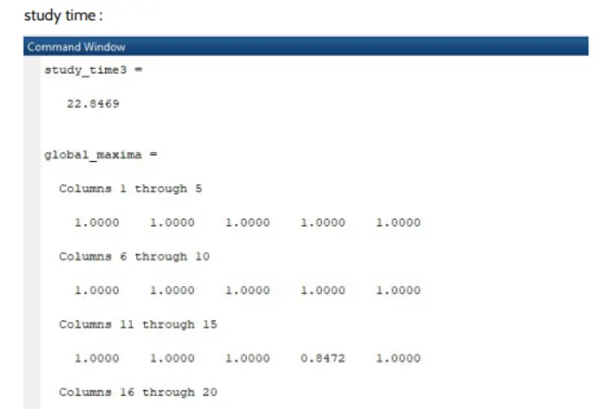
STUDY TIME :
CONCLUSION:
Finally we finded an global maxima of the function and we got all 3 studies and for F maxima vs no.of itterations.