Project 2 - Rankine cycle Simulator
Rankine cycle - Basic process description
The rankine cycle is the fundamental operating cycle of all power plants where an operating fluid is continously evaporated and condensed. The selection of operating fluid depends mainly on the available temperature of range. The Rankine cucle is idealized thermodynamic cycle of a constant pressure heat engine that converts part of heat into mechanical work.
In this cycle heat is supplied externally to a closed loop, which is usually uses water as the water fluid.
| 1-2; | Isentropic Compression |
Waters enters the pump at state 1 as satuurated liquid and is compressed isentropically to the operating pressure of boiler. |
| 2-3; | Constant P heat addition | Saturated water enters the boiler and leaves it as superheated vapour at state 3. |
| 3-4; | Isentropic Exprression | Superheated vapour expands isentropically in turbine and produce work. |
| 4-1; | Constant P heat Rejection | High quality steam is condensed in the condenser. |
RANKINE CYCLE DIAGRAM:
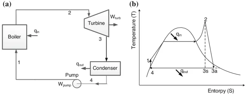
The components used in Rankine Cycle are
1.Boiler
2. Pump
3.Condenser
4. Steam turbine
These are the main components used in Rnkine Cycle.
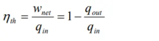
Thermal Efficiency of Rankine Cycle:
Program Description:
Step 1: % Cleaning the command window and clearing all windows by using the command clear all close all clc.
Step 2: In the second step we use fprintf command was used to display the process in the command window as per the required output provided. 'n' is the command used to represent new line.
Step 3: In this step the 'input' command is used to ener the variables of turbine inlet pressure, turbine inlet temperature and pressure at the condenser.
Step 4: In this step the fallowing variable at stages 1,2,3,4,5 and 6 were evaluated from Xstream file provided.
Step 5: In this final step the Figure Command is used to geneerate the plot with x label and ylabel to provide labels to the graphical representation of x-axis and y-axis.
Main Code:
clear all
close all
clc

%displaying the process in different stages
fprintf('RANKINE CYCLE SIMULATORn')
fprintf('Isentropic Expansion in the Turbine n')
fprintf('Constant Pressure Heat Rejection by the Condenser')
fprintf('Isentropic Compression in the pump')
fprintf('Constant pressure Heat Addition by the Boiler')

%To enter the input for state point calculation
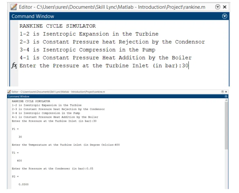
P1=input('Enter the pressure at the Turbine Inlet (in bar):')
T1=input('Enter the temperature at the Turbine inlet (in degree celcius):')
P2=input('Enter the pressurer at the condenser(in bar):')

%to calculate steam point values-state point 1
H1=Xsteam('h_PT',P1,T1)% Enthalpy at state point 1
S1=Xsteam('s_PT',P1,T1)% Entropy at state point 1

%to calculate state point values - state point 2&3
S2=S1;
P3=P2; % constant pressurre heaat rejection in condenser
s_f2=Xsteam('sL_p',P2);
s_g2=Xsteam('sV_p',P2);
h_f2=Xsteam('hL_p,P2');
h_g2=Xsteam('hV_p,P2');
S3=Xsteam('sL_P',P3);
H3=Xsteam('hL_P',P3);
T2=Xsteam('Tsat_p',P3);
T3=T2;
H2=h_g2;

%to calculate the state point values - state point  4
S4=S3;%Isentropic compression
P4=P3;%Constaant prressure
T4=XSteam('T_ps',P4,S4);
H4=XSteam('h_pT',P4,S4);
H4_1=XSteam('hL_P',P4);
S4_1=XSteam('sL_P',P4);
H4_2=XSteam('sV_P',P4);
S4_2=XSteam('sV_P',P4);
T4_1=XSteam('T_hs',H4_1,S4_1);
T4_2=XSteam('T_hs',H4_2,S4_2);

%Work done in turbine
Wt=H1-H2;
%Work done in pump
Wp=H4-H3;
%net work done
Wnet=Wt-Wp
%thermal efficiency
Q1=H1-H4;% Heat addition to the system
Q2=H2-H3;% Heat rejection from the system
Ntherma=((Wt-Wp)/Q1)*100;
% Specific steam consumption
SSC=(3600/Wnet);

% to calculating T,S,and H at the vapour and liquid
T6=XSteam('Tsat_p',P1);
S5=XSteam('sL_p',P1);
S6=XSteam('sV_P',P1);
H5=XSteam('hL_p',P1);
H6=XSteam('hV_P',P1);
T5=T6;

%Printing the output to command window
fprintf('n RESULT n')
fprintf('At state point 1: np1 is : %4.2f nT1 is : %4.2f Degree celcius nH1 is : %4.2f kJ/KgnS1 is : %4.2f kJ/kgknn',P1,T1,H1,S1)
fprintf('At state point 2: np2 is : %4.2f nT2 is : %4.2f Degree celcius nH2 is : %4.2f kJ/KgnS2 is : %4.2f kJ/kgknn',P2,T2,H2,S2)
fprintf('At state point 3: np3 is : %4.2f nT3 is : %4.2f Degree celcius nH3 is : %4.2f kJ/KgnS3 is : %4.2f kJ/kgknn',P3,T3,H3,S3)
fprintf('At state point 4: np4 is : %4.2f nT4 is :%4.2f Degree celcius nH4 is : %4.2f kJ/KgnS4 is : %4.2f kJ/kgknn',P4,T4,H4,S4)
fprintf('Wt is :%4.2f kJ/kgnWp is : %4.2f kJ/KgnWnet is : %4.2f kJ/kgNtherm is :4.2f percentnS.S.C is : 4.2f kg/kWh',Wt,Wp,Wnet,Ntherm,SSC)

temperature_ranges=linspace(0,550,1000);
for i=1:length(temperature_ranges(i));
    s_v(i)=XSteam('sV_T',temperature_ranges(i));
    s_l(i)=XSteam('sL_T',temperature_ranges(i));
    h_v(i)=XSteam('hV_T',temperature_ranges(i));
    h_v(i)=XSteam('hV_T',temperature_ranges(i));
end

%To plot Entropy and Temperature
figure(1)
plot([S1 S2],[T1 T2],[S2 S3],[T2 T3],[S3 S4],[T3 T4],[S5 S6],[T5,T6],[S6 S1],[T6 T1],[S4 S4_1],[T4 T4_1],[S4_1 S4_2],[T4_1 T4-2][S4_2 S4_1][T4_2 T4_1],'Marker','o,'color','b','Linewidth',2)
hold on
plot(s_v,temperature_ranges)
plot(s_l,temperature_ranges)
xlabel('Entropy S [kJ/Kg/K] '); %X  axis label
ylabel('Temperatures T [K] ');%y axis   label
title('Temperature(T) - Entropy(S) plot') %title for the plot

%To plot Entropy and Enthalpy
figure(2)
plot([S1 S2],[H1 H2],[S2 S3],[H2 H3],[S3 S4],[H4 H3],[S4 S1],[H4 H1],'marker','o','Color','r','LineWidth',2)
hold on
plot(s_v,h_v)
plot(s_l,h_l)
xlabel('Entropy S [kJ/KgK] ');%x axis label
ylabel('Enthalpy H [kJ/K] ');%y axis label
title('Enthalpy(H) - Entropy(S) plot ')%title for the plot
CODE EXPLANATION:
- First we want to clear the command window by using clear all close all clc.
- Now give the rankine cycle process and what are the steps involved in the process and excitue the steps.
- Now give the inputs of pressure and temperature for the rankine cycle.
- After giving inputs to the rankine cycle calcute the states vise.
- To calculate the states we need enthalpy and entropy for the process.
- So through the help of Xsteam data file we got values of enthalpy and entropy values to calculate the rankine cycle.
- Now find the work done for the cycle and work out put and work efficiency.
- Finally we need to find the Thermal Efficiency of the rankine cycle.
- Now use plot command and give the plots for xlabel and ylabel.
- We want to give two plottings one for etropy and temperature and second plot for entropy and enthalpy.
- Finally give tittle for the xlabel and ylabel and run the command.
INPUTS GIVEN IN COMMAND WINDOW:
OUT PUT RESULTS FOR COMMAND WINDOW:
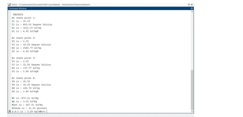
All state variables at different stages from 123 and 4 were determined and exicuted.
Net work out put is: 667.01 kJ/kg
PLOT OUTPUT
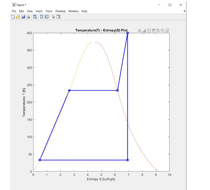
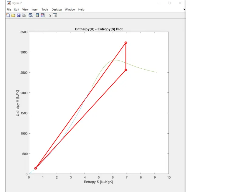
The T-S and S-H were plotted for the rankine cycle using Xsteam data file where the process is isobaric heat transfer or constant pressure heat addition to the system.
CONCLUSION: Finally we finded an thermal effficiency of the rankine cycle and we plotted the output for the T-S and H-S for the rankine cycle.
REFERNCES: