Project 2 - Rankine cycle Simulator

AIM:

• To Understand the concept of Rankine cycle by referring to standard thermal engineering text book and to create a rankine cycle simulator using matlab.

OBJECTIVE :

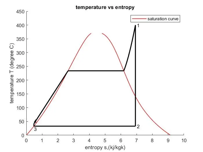
• To plot T-S diagram for the rankine cycle
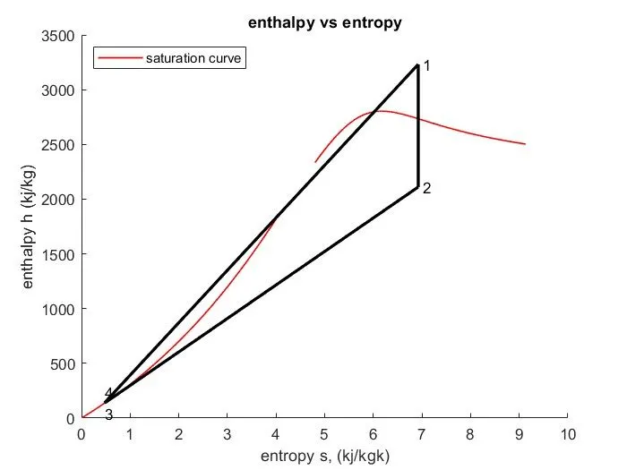
• To plot H-S diagram for the rankine cycle
• To obtain state points by referring Xsteam data library given

RANKINE CYCLE :

Process diagram :

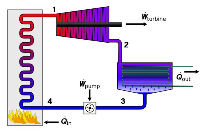
Rankine cycle consists of following components

• TURBINE
• CONDENSER
• PUMP
• BOILER

Rankine cycle is a vapour powered cycle where dry saturated vapour is working fluid. Here Ideal rankine cycle is considered where the cycle operates without irreversiblity and frictional pressure loses at each stages. Water is used as it has many advantages like more abundant , less toxic, low cost.. etc. Ideal Rankine cycle has 4 stages

Rankine cycle

PROCESS 1-2

TURBINE: process 1-2 performs in turbine where the dry saturated vapour hits the turbine blades , here the mechanical energy of the blades is converted into electrical energy. It performs under isentropic expansion, Where the temperature and pressure gets reduced

PROCESS 2-3

CONDENSER: process 2-3 performs in condenser, here the vapour gets condensed in condenser at constant pressure, the condensation takes out the heat and sends it to pump.

PROCESS 3-4

PUMP: process 3-4 takes in pump where the liquid after condensation compressed to high pressure in pump carried out under isentropic compression state.

PROCESS 4-1

BOILER: process 4-1 is boiling the high pressure liquid to saturation temperature in a boiler with the help of external fuel like coal, natural gas fuel..etc. It is done by constant pressure heat addition.

THE CODE:

clear all
close all
clc

%displaying process followed in rankine cycle
disp('RANKINE CYCLE');
disp('1-2 isentropic expansion occurs in turbine');
disp('2-3 heat rejection at constant pressure in condenser');
disp('3-4 isentropic compression at pump');
disp('4-1 heat adiition at constant pressure in boiler');

%gettig inputs 
p1 = input('\n turbine inlet pressure,p1 in bar = ');
t1 = input('\n temperature at inlet of turbine, ti in degree celcius = ');
p2 = input('\n inlet pressure at condenser, p2 in bar = ');

% defining variables at 4 states

%satate 1
h1 = XSteam('h_pT', p1, t1);  %enthalphy as a function of pressure amd temperature
s1 = XSteam('s_pT', p1 ,t1);  %entropy as a function of pressure amd temperature

%state 2
s2 = s1;
sf2 = XSteam('sL_p', p2 );
sg2 = XSteam('sV_p', p2);
x2 = (s2 - sf2)/(sg2-sf2);
hf2 = XSteam('hL_p', p2);
hg2 = XSteam('hV_p', p2);
h2 = hf2 + (x2*(hg2-hf2));

%state 3
p3 = p2;
s3 = XSteam('sL_p', p3);
h3 = XSteam('hL_p', p3);

%state 4
p4 = p1;
s4 = s3;
 
% work done in turbine
Wt = h1 - h2;

% work done in pump
v3 = XSteam('vL_p', p3);
Wp = v3*(p4 - p3)*100;
h4 = Wp + h3;

% net work
Wnet = Wt - Wp;

% heat into the sysytem
Qin = h1 - h4;

% heat out from the system
Qout = h2 - h3;

% thermal efficiency
EF =(Wnet/Qin)*100;

%SPECIFIC STEAM consumption rate
%ssc= mass flow rate/ power
ssc = (3600/Wnet);

%back work ratio
bwr =(Wp/Wt);

% temperature at state points
t3 = XSteam('Tsat_p', p3);
t2 = t3;
cp4 = XSteam('Cp_ps', p4, s4);
cv4 = XSteam('Cv_ps', p4, s4);
k = cp4/cv4;
t4 = t3/((p3/p4)^((k-1/k)));

%calculating temperature, enthalpy and entropy at vapour and liquid phases
%for plotting
t6 = XSteam('Tsat_p',p1);
s5 = XSteam('sL_p', p1);
s6 = XSteam('sV_p', p1);
h5 = XSteam('hL_p', p1);
h6 = XSteam('hV_p', p1);
t5 = t6;

% saturation curve
t = linspace(1,370,1000);
for i = 1:length(t)

    sg(i) = XSteam('sV_T', t(i));
    sf(i) = XSteam('sL_T', t(i));
    hg(i) = XSteam('hV_T', t(i));
    hf(i) = XSteam('hL_T', t(i));
end

%plotting T -S diagram
figure(1)
hold on
plot(sf, t,'r','lineWidth',1);
plot(sg, t,'r','lineWidth',1);
plot([s1 s2], [t1 t2], 'k','linewidth',2);
plot([s2 s3], [t2 t3], 'k','linewidth',2);
plot([s3 s4], [t3 t4], 'k','linewidth',2);
plot([s4 s5], [t4 t5], 'k','linewidth',2);
plot([s5 s6], [t5 t6], 'k','linewidth',2);
sc1 = linspace(s6,s1,1000);
for l = 1 :length(sc1)
    tc1(l) = XSteam('T_ps', p1, sc1(l))
end
plot(sc1, tc1,'k','linewidth', 2);
text(s1+0.1,t1,'1')
text(s2+0.1,t2,'2')
text(s3,t3-10,'3')
text(s4,t4+10,'4')
title('temperature vs entropy')
xlabel('entropy s,(kj/kgk)')
ylabel('temperature T (degree C)')
legend('saturation curve')

%plotting enthalpuy and entropy
figure(2)
hold on 
plot(sf, hf,'r','lineWidth',1);
plot(sg, hg,'r','lineWidth',1);
plot([s1 s2], [h1 h2] , 'k', 'lineWidth',2);
plot([s2 s3], [h2 h3] , 'k', 'lineWidth',2);
plot([s3 s4], [h3 h4] , 'k', 'lineWidth',2);
plot([s4 s1], [h4 h1] , 'k', 'linewidth',2);
text(s1+0.1,h1,'1')
text(s2+0.1,h2,'2')
text(s3,h3-100,'3')
text(s4,h4+100,'4')
title('enthalpy vs entropy')
xlabel('entropy s, (kj/kgk)')
ylabel('enthalpy h (kj/kg)')
legend('saturation curve', 'Location','northwest')

%displaying results in command window
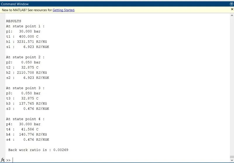
disp('RESULTS')
fprintf('At state point 1 : \n');
fprintf('p1: %8.3f bar\n', p1);
fprintf('t1 : %8.3f C\n', t1);
fprintf('h1 : %8.3f KJ/KG\n', h1);
fprintf('s1 : %8.3f KJ/KGK\n\n', s1);

%state point 2
fprintf('At state point 2 : \n');
fprintf('p2: %8.3f bar\n', p2);
fprintf('t2 : %8.3f C\n', t2);
fprintf('h2 : %8.3f KJ/KG\n', h2);
fprintf('s2 : %8.3f KJ/KGK\n\n', s2);

%state point 3
fprintf('At state point 3 : \n');
fprintf('p3: %8.3f bar\n', p3);
fprintf('t3 : %8.3f C\n', t3);
fprintf('h3 : %8.3f KJ/KG\n', h3);
fprintf('s3 : %8.3f KJ/KGK\n\n', s3);

%state point 4
fprintf('At state point 4 : \n');
fprintf('p4: %8.3f bar\n', p4);
fprintf('t4 : %8.3f C\n', t4);
fprintf('h4 : %8.3f KJ/KG\n', h4);
fprintf('s4 : %8.3f KJ/KGK\n\n', s4);

fprintf(' Back work ratio is : %2.5f\n\n',bwr);

CODE EXPLANATION:

First clear all, close all, clc is used to close the back stuffs and to start a new program.

The code 'disp' is used to display the coded contents in command window. Following this code the process carried out in rankine cycle is made to display in the command window by specifying each stage process using 'disp'.

Getting input data to solve the problem using 'input' command. It is used similar to disp command by speciying the contents after 'input' command. Here p1, t1, t2 are the input data given to solve the problem. Doing this is done for simulator level problems as the code asks the input value after executing the program.

After getting input data the thermodynamic entities at state point variables are refrred from the Xsteam data library given .

This is used to obtain the state point s,h,t by giving in any of the dependent variable for determining it.This is done by Xsteam(' ', , )where the ' ' recognises the variable undergoing the thermodynamic state like saturated, vapourised, liquified...etc, Xsteam(' ', , ) pos 2 and 3 refers to the dependent variable like pressure,temperature.

By referring Xsteam data all the state points are referred and approached in classical mathematical solving method

Wpump = h4-h3 : WORK DONE BY THE PUMP

Wt = h1-h2 : WORK DONE BY THE TURBINE

heat given to system : Qin = h1-h4

heat taken from the system : Qout = h3-h2

CONCLUSION:

The plot T-S diagram has been plotted with saturation curve , here only 4 state points are mentioned as the curve intersects at other two points . These two points are undergoing inside boiler itslef

The plot H-S diagram has been plotted withn saturation curve

Back work ratio has been found out

Wnet is found out

Simulator mode of problem solving is done for The Rankine cycle.

PLOTS:

t-s diagram

plot h-s diagram

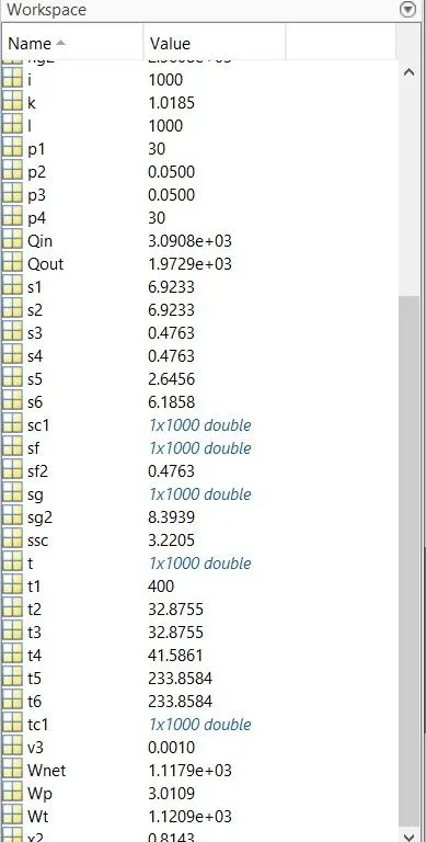
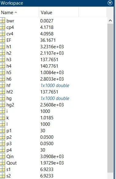
screenshots: