Week 3 - Taylor table method and Matlab code
AIM-To derive the second order derivative using central difference, Skewed right-sided difference and Skewed left-sided difference and write a program in matlab to find the deviation from the analytical derivate and plot it in a graph, also plot forward and bacward difference from the same and plot in graph.
OBJECTIVE -
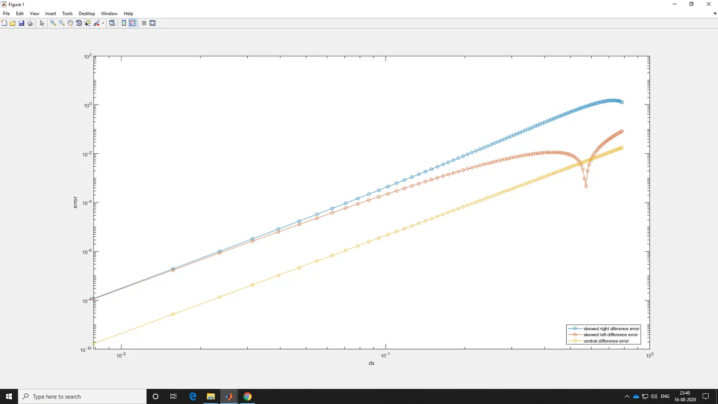
a. Provide a plot that compares the absolute error between the above-mentioned schemes
b. In your own words, describe why a skewed scheme is useful? What can a skewed scheme do that a CD scheme cannot do?
4. Paste your code using the "INSERT CODE SAMPLE" option and explain your outputs.
5. Write a detailed explanation for your results, plots or codes without explanation will award zero marks.
FORMULA
Central difference
`f''(x)=(a*f(i-2)+b*f(i-1)+c*f(i)+d*f(i+1)+e*f(i+2))/(Delta x^2)`
Skewed right-sided difference
`f''(x)=(a*f(i)+b*f(i+1)+c*f(i+2)+d*f(i+3)+e*f(i+4)+g*f(i+4))/(Delta x^2)`
Skewed left-sided difference
`f''(x)=(a*f(i-5)+b*f(i-4)+c*f(i-3)+d*f(i-2)+e*f(i-1)+g*f(i))/(Delta x^2)`
TAYLOR TABLE
Skewed right-sided difference
`[[Deltax^2f''(i), f(i),Deltaxf(i),Deltax^2f(i),Deltax^3f'''(i),Deltax^4f^(iv)(i), Deltax^5f^(v)(i)],[af(i),a,0,0,0,0,0],[bf(i+1),b,b,b/2,b/6,b/24,b/120],[cf(i+2),c,2c,(4c)/2,(8c)/6,(16c)/24,(32c)/120],[df(i+3),d,2d,(9d)/2,(27d)/6,(81d)/24,(243d)/120 ],[ef(i+4),e,4e,(16e)/2,(64e)/6,(256e)/24,(1024)/120],[gf(i+5),g ,g,(25g)/2,(125g)/6,(625g)/24,(3125g)/120],[ Deltax^2f''(i),0,0,1,0,0,0]]`
Central difference
`[[Deltax^2f''(i), f(i),Deltaxf(i),Deltax^2f(i),Deltax^3f'''(i),Deltax^4f^(iv)(i), Deltax^5f^(v)(i)],[af(i-2),a,2a,(4a)/2,(8a)/6,(16a)/24,(32a)/120],[bf(i-1),b,b,b/2,b/6,b/24,b/120],[cf(i),c,0,(0),(0),(0),(0)],[df(i+1),d,d,d/2,d/6,d/24,d/120 ],[cf(i+2),c,2c,(4c)/2,(8c)/6,(16c)/24,(32c)/120]]`
Skewed left-sided difference
`[[Deltax^2f''(i), f(i),Deltaxf(i),Deltax^2f(i),Deltax^3f'''(i),Deltax^4f^(iv)(i), Deltax^5f^(v)(i)],[af(i-5),a ,a,(25g)/2,(125a)/6,(625a)/24,(3125a)/120],[bf(i-4),b,4b,(16b)/2,(64b)/6,(256b)/24,(1024b)/120],[cf(i-2),c,2c,(4c)/2,(8c)/6,(16c)/24,(32c)/120],[df(i-3),d,2d,(9d)/2,(27d)/6,(81d)/24,(243d)/120 ],[ef(i-1),b,b,b/2,b/6,b/24,b/120],[f(i),a,0,0,0,0,0],[ Deltax^2f''(i),0,0,1,0,0,0]]`
CODE
close all
clear
clc

%finding the values of constants for skewed right sided difference
%assigning the coefficients in the matrix form
a_right_skewed=[1,1,1,1,1,1;0,1,2,3,4,5,;0 1/2 4/2 9/2 16/2,25/2 ;0 1/6 8/6 27/6 64/6,125/6 ;0 1/24 16/24 81/24 256/24,625/24;0,1/120,32/120,243/120,1024/120,3125/120 ];
%assigning the results of the equation in matrix form
b_right_skewed=[0;0;1;0;0;0];
%finding the constants and add in a matrix
x_right_skewed=inv(a_right_skewed)*b_right_skewed;

%finding the values of constants for skewed left sided difference
%assigning the coefficients in the matrix form
a_left_skewed=[1,1,1,1,1,1;-5,-4,-3,-2,-1,0;25/2,16/2,9/2,4/2,1/2,0;-125/6,-64/6,-27/6,-8/6,-1/6,0;625/24,256/24,81/24,16/24,1/24,0;-3125/120,-1024/120,-243/120,-32/120,-1/120,0];
%assigning the results of the equation in matrix form
b_left_skewed=[0;0;1;0;0;0];
%finding the constants and add in a matrix
x_left_skewed=inv(a_left_skewed)*b_left_skewed;

%finding the values of constants for central difference
%assigning the coefficients in the matrix form
a_central=[1,1,1,1,1; -2,-1,0,1,2;4/2,1/2,0,1/2,4/2;-8/6,-1/6,0,1/6,8/6;16/24,1/24,0,1/24,16/24];
%assigning the results of the equation in matrix form
b_central=[0;0;1;0;0];
%finding the constants and add in a matrix
x_central_skewed=inv(a_central)*b_central;

%value of x
x=pi/3;
%value of the difference
dx=linspace(pi/4,pi/400);

%the value of the analytical derivative exp(x)*cos(x)=-2*sin(x)*exp(x)
analytical=-2*sin(x)*exp(x);

for i=1:length(dx)

%solving the matrix the formula to calculate the output
%f''(x)=(exp(x)*cos(x)+exp(x+i)*cos(x+i)+exp(x+2i)*cos(x+2i)+exp(x+3i)*cos(x+3i)+exp(x+4i)*cos(x+4i)+exp(x+5i)*cos(x+5i))/dx^2
%here we break the equations to r1 r2 r3 r4 r5 r6
r1(i)=(exp(x).*cos(x));
r2(i)=(exp(x+dx(i)).*cos(x+dx(i)));
r3(i)=(exp(x+2*dx(i)).*cos(x+2*dx(i)));
r4(i)=(exp(x+3*dx(i)).*cos(x+3*dx(i)));
r5(i)= (exp(x+4*dx(i)).*cos(x+4*dx(i)));
r6(i)= (exp(x+5*dx(i)).*cos(x+5*dx(i)));
right_skewed(i)=(x_right_skewed(1,1).*r1(i)+x_right_skewed(2,1).*r2(i)+x_right_skewed(3,1).*r3(i)+x_right_skewed(4,1).*r4(i)+ x_right_skewed(5,1).*r5(i)+x_right_skewed(6,1).*r6(i))/(dx(i)^2);


%solving the matrix the formula to calculate the output
%f''(x)=(exp(x)*cos(x)+exp(x-i)*cos(x-i)+exp(x-2i)*cos(x-2i)+exp(x-3i)*cos(x-3i)+exp(x-4i)*cos(x-4i)+exp(x-5i)*cos(x-5i))/dx^2
%here we break the equations to l1 l2 l3 l4 l5 l6
 l1(i)=(exp(x-5*dx(i)).*cos(x-5*dx(i)));
 l2(i)=(exp(x-4*dx(i)).*cos(x-4*dx(i)));
 l3(i)=(exp(x-3*dx(i)).*cos(x-3*dx(i)));
 l4(i)=(exp(x-2*dx(i)).*cos(x-2*dx(i)));
 l5(i)=(exp(x-dx(i)).*cos(x-dx(i)));
 l6(i)=(exp(x).*cos(x));
left_skewed(i)=(x_left_skewed(1,1).*l1(i)+x_left_skewed(2,1).*l2(i)+x_left_skewed(3,1).*l3(i)+x_left_skewed(4,1).*l4(i)+x_left_skewed(5,1).*l5(i)+x_left_skewed(6,1).*l6(i))/(dx(i)^2);

%solving the matrix the formula to calculate the output
%f''(x)=exp(x-2i)*cos(x-2i)+exp(x-i)*cos(x-i)+exp(x)*cos(x)+exp(x+1i)*cos(x+1i)+exp(x+2i)*cos(x+2i))/dx^2
y=x_central_skewed(1,1)*(exp(x-2*dx(i))*cos(x-2*dx(i)))+x_central_skewed(2,1)*(exp(x-1*dx(i)).*cos(x-1*dx(i)))+x_central_skewed(3,1)*(exp(x)*cos(x))+x_central_skewed(4,1)*(exp(x+1*dx(i))*cos(x+1*dx(i)))+x_central_skewed(5,1)*(exp(x+2*dx(i))*cos(x+2*dx(i)));
central_difference(i)=y/(dx(i)^2);

%taking the values from the skewed right and left respectively and finding the forward and backward difference
forward=(r2(i)-r1(i))./dx;
backward=(l6(i)-l5(i))./dx;

%calculating the errors
%error for the skewed right sided difference
error_1(i)=abs((analytical-right_skewed(i))/analytical);
%error for the skewed left sided difference
error_2(i)=abs((analytical-left_skewed(i))/analytical);
%error for the skewed central difference
error_3(i)=abs((analytical-central_difference(i))/analytical);
%error for the forward difference
error_4(i)=abs((analytical-forward(i))/analytical);
%error for the backward difference
error_5(i)=abs((analytical-backward(i))/analytical);

end

%plotting the figure and comparing the error between analytical derivative
figure(1)
loglog(dx,error_1,'o-');
hold on;
loglog(dx,error_2,'o-');
loglog(dx,error_3,'o-');
xlabel('dx');
ylabel('error');

legend('skewed right diference error','skewed left difference error','central difference error','location','best');

%forward and backward difference
figure(2)

loglog(dx,error_4,'o-');
hold on;
loglog(dx,error_5,'o-');
legend('forward difference error','backward difference error','location','best');
xlabel('dx');
ylabel('error');
OUTPUT
PLOT FOR Central difference,Skewed right-sided difference, Skewed left-sided difference
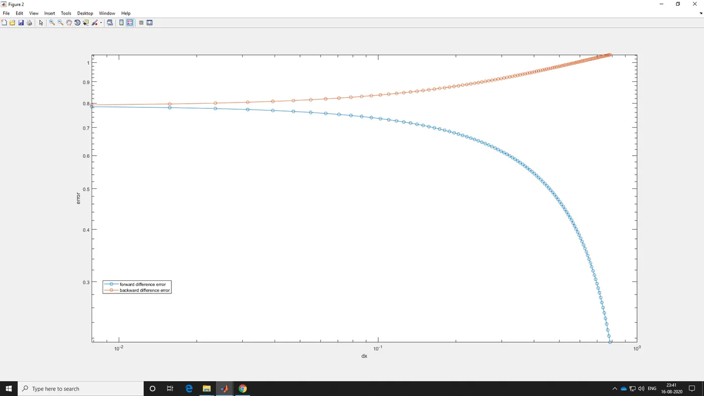
PLOT FOR FORWARD AND BACKWARD DIFFERENCE
DESCRIPTION
In skewed scheme the values next to the known value can be obtained by knowing a single value or initial value, so it is reliable.
For an central difference the values before and after the given value is required to approximate the unknown values so minimum two values are necessary to approximate the unknown.