Week 3 - Taylor table method and Matlab code

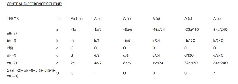
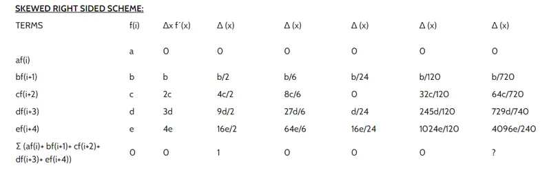
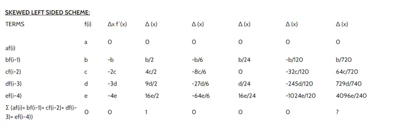
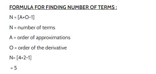
AIM: To derive the following 4th order approximations of the second-order derivative.

1. Central difference

2. Skewed right-sided difference

3. Skewed left-sided difference

and writing a program in Matlab to evaluate the second-order derivative of the analytical function exp(x)*cos(x) and compare it with the 3 numerical approximations.

PROCEDURE: Derivation of fourth order approximations for second order derivative. Taylor tables are shown:

MATLAB Code to derive the second order derivative of the given function and comparing the result using different schemes:

clear all
close all
clc

%values for x and dx
x = pi/4;
dx = linspace(pi/4,pi/4000,20);

for i = 1: length(dx)

 central_error(i) = central_diff_approximation(x, dx(i));  %Error by central differencing
 
 rightskewed_error(i) = rightskewed_approximation(x, dx(i));  %Error by skewed right sided differencing
 
 leftskewed_error(i) = leftskewed_approximation(x,dx(i));  %Error by skewed left sided differencing
 
 fds_error(i) = forward_approximation(x,dx(i));  %Error by forwad differencing
 
 bds_error(i) = backward_approximation(x,dx(i));  %Error by backward differencing
 
end  

%plotting the dx values against errors for each type of approximation
figure(1)
loglog(dx, central_error,'linewidth',2)
hold on
loglog(dx, rightskewed_error, 'r','linewidth',2)
hold on
loglog(dx, leftskewed_error,'g','linewidth',2)
hold on
loglog(dx, fds_error, 'y','linewidth',2)
hold on
loglog(dx, bds_error,'linewidth', 2)
grid
xlabel('dx')
ylabel('Absolute error')
legend('Central error', 'Right skewed error', 'Left skewed error', 'FDS error', 'BDS error')

Function Code for Central Difference scheme:

%Function for central differencing scheme 

function out = central_diff_approximation(x, dx)
  
  %f(x) = exp(x)*cos(x)
  %Analytical derivative = f'(x) = -2*exp(x)*sin(x) 
  
  analytical_derivative = -2*exp(x)*sin(x);
  
  % numerical derivative
  %fourth order central differencing approximation
  a = -0.0833;
  b = 1.3333;
  c = -2.5000;
  d = 1.3333;
  e = -0.0833;
  %central_differencing = (a*f(i-2) + b*f(i-1)+ c*f(i) +d*f(i+1) + e*f(i+2))/?x^2
  
 central_differencing = ((a*exp(x-(2*dx))*cos(x-(2*dx))) + (b*exp(x-dx)*cos(x-dx))+ (c*exp(x)*cos(x)) + (d*exp(x+dx)*cos(x+dx)) + (e*exp(x+(2*dx))*cos(x+(2*dx))))/(dx^2);
 
 %output
     out = abs(central_differencing - analytical_derivative)

end

Function for right skewed difference scheme:

%Function for Skewed right sided differencing scheme 

function out = rightskewed_approximation(x, dx)
  
  %f(x) = exp(x)*cos(x)
  %Analytical derivative = f'(x) = -2*exp(x)*sin(x) 
  
  analytical_derivative = -2*exp(x)*sin(x);
  
  % numerical derivative
  %fourth order Skewed right sided differencing approximation
  a = 3.75000;
  b = -12.83333;
  c = 17.83333;
  d = -13.0000;
  e = 5.08333;
  h = -0.83333;
  %rightskewed_differencing = ( a*f(i) + b*f(i+1)+ c*f(i+2) +d*f(i+3) + e*f(i+4) + h*f(i+5))/?x^2
  
 rightskewed_differencing = ((a*exp(x)*cos(x)) + (b*exp(x+dx)*cos(x+dx))+ (c*exp(x+(2*dx))*cos(x+(2*dx))) + (d*exp(x+(3*dx))*cos(x+(3*dx))) + (e*exp(x+(4*dx))*cos(x+(4*dx))) + (h*exp(x+(5*dx))*cos(x+(5*dx))))/(dx^2);
 
 %output
     out = abs(rightskewed_differencing - analytical_derivative)

end

Function for left skewed difference scheme:

%Function for Skewed left sided differencing scheme 

function out = leftskewed_approximation(x, dx)
  
  %f(x) = exp(x)*cos(x)
  %Analytical derivative = f'(x) = -2*exp(x)*sin(x) 
  
  analytical_derivative = -2*exp(x)*sin(x);
  
  % numerical derivative
  %fourth order Skewed left sided differencing approximation
  a = -0.83333;
  b = 5.08333;
  c = -13.00000;
  d = 17.83333;
  e = -12.83333;
  h = 3.75000;
  %leftskewed_differencing = ( h*f(i) + e*f(i-1)+ d*f(i-2) +c*f(i-3) + b*f(i-4) + a*f(i-5))/dx^2
  
 leftskewed_differencing = ((h*exp(x)*cos(x)) + (e*exp(x-dx)*cos(x-dx))+ (d*exp(x-(2*dx))*cos(x-(2*dx))) + (c*exp(x-(3*dx))*cos(x-(3*dx))) + (b*exp(x-(4*dx))*cos(x-(4*dx))) + (a*exp(x-(5*dx))*cos(x-(5*dx))))/(dx^2);
 
 %output
     out = abs(leftskewed_differencing - analytical_derivative)

end

Error through forward difference scheme-Function:

%Function for Forward differencing scheme 

function out = forward_approximation(x, dx)

   %f(x) = exp(x)*cos(x)
  %Analytical derivative = f'(x) = -2*exp(x)*sin(x) 
  
  analytical_derivative = -2*exp(x)*sin(x);
  
  % numerical derivative
  % forward_differencing = (f(x+dx) -  f(x))/dx
   
    forward_differencing = ((exp(x+dx)*cos(x+dx)) - (exp(x)*cos(x)))/dx; 
   

    %output
     out = abs(forward_differencing - analytical_derivative)
  
  end

Error through Backward difference scheme-Function:

%Function for Backward differencing scheme 

function out = backward_approximation(x, dx)

   %f(x) = exp(x)*cos(x)
  %Analytical derivative = f'(x) = -2*exp(x)*sin(x) 
  
  analytical_derivative = -2*exp(x)*sin(x);
  
  % numerical derivative
  % backward_differencing = (f(x-dx) -  f(x))/dx
   
    backward_differencing = ((exp(x-dx)*cos(x-dx)) - (exp(x)*cos(x)))/dx; 
   

    %output
     out = abs(backward_differencing - analytical_derivative)
  
  end

Results and Plots:

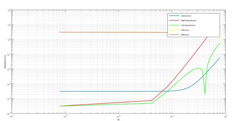
The error comparision between all the schemes for the given funtion is shown:

Conclusions:

Conclusion

• From the above plot it is clear that the fourth order differencing approaches are very much more accurate than the first order difference approaches like FDS and BDS. When dx is being reduced, fourth order approximations get closer to the exact value in an accelerated rate. Hence higher order approximations are significantly more accurate than first order approximations.
• When comparing the fourth order approximations, we find that the skewed difference scheme gives the lowest errors than the central difference scheme. With the decrease in dx value, the errors of skewed difference schemes are also reducing. But for the central difference scheme, after some point, the error value is a constant even after further reduction in dx value.
• At times when there are no nodes on anyone of the either sides of the node we consider to discretize, we cannot use central differece scheme because it requires informations from nodes of either sides. In this type of situations, skewed difference schemes are useful because they require information only from any one of the sides of the node under consideration.