Week 3 - Solving second order ODEs

Solving second order ODEs

AIM: Simulate the transient behavior of the simple pendulum and the animation is created.

THEORY:

Ordinary differential equations:

An ordinary differential equation (ODE), in Mathematics, is an equation that consists of one or more functions of one independent variable along with their derivatives. A differentis an equation that contains a function with one or more derivatives. But in the case ODE, the word ordinary is used for the derivative of the functions for the single independent variable.

Simple Pendulum:

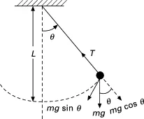
The simple pendulum is another mechanical system that moves in an oscillatory motion. It consists of a point mass 'm' suspended by means of a light inextensible string of length L from fixed support as shown in Fig. The motion occurs in a vertical plane and is driven by a gravitational force. The forces which are acting on the mass are shown in the figure. The tangential component of the gravitational force, mg sin θ, always acts towards the mean position θ = 0 opposite to the displacement, restoring force acting tangent to the arc.

EQUATIONS USED:

The secound order ODE for a simple pendulum:

`(d^2theta)/(dt^2)+b/m*(d theta)/dt+g/l*sin theta = 0`

Where

b = Damping cofficient

m = Mass of the bob(kg)

g = Accelaration due to gravity

L = Length of the rod(m)

TO change the ODE `2^(nd)`order to `1^(st)`order

let `theta=theta_1`

`(d theta)/(dt) = (d theta_1)/dt = theta_2`

`(d^2 theta)/dt^2 = (d^2 theta_1)/dt^2=d/dt((d theta_1)/dt) = (d theta_2)/dt`

From above equations

`(d^2 theta_1)/dt^2 +b/m*(d theta_1)/dt+g/L*sin theta_1 = 0`

`(d theta_2)/dt^2+b/m*theta_2+g/L*sin theta_1 = 0`

`(d theta_2)/dt = -b/m*theta_2-g/L*sin theta_1`

To arrangement in the matrix form

`(d theta)/dt` = `d/dt``[ [theta_1],[theta_2] ]``[ [theta_2],[-b/m*theta_2-g/L*sin theta_1] ]`

Explanation:

• Initially, the pre-input values given such as damping coefficient, the center of gravity, length of the spring, the mass of the ball.
• The angular displacement and angular velocity is taken as input angkes
• time is given from 0 to 20 sec for 500 frames.
• ODE functions created using to mentioned formula
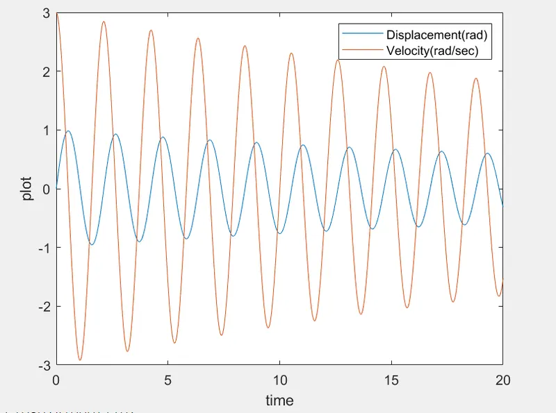
• the graph is plotted angular displacement, angular velocity vs time.
• To show a simulation of the pendulum 'for loop' is used to continuously plot the graph showing the pendulum
• used video writer to create the movie
• the animation opened, written, and closed to provide an animation continuously

CUDE:

clear all
close all
clc            

%initial input values
b = 0.05;    % Damping cofficient
g = 9.81;    % centre of gravity in m/s^2
l = 1;       % Length of the string
m = 1;       % mass of a ball in kg

%initial condtion
theta_0 = [0;3]; %[angula displacement, angular velocity]

%time points
t_span = linspace (0,20,500);

%solve ODE
[t,results] = ode45(@(t,theta) ode_func(t,theta,b,g,l,m), t_span, theta_0);

plot(t,results(:,1))
hold on
plot(t,results(:,2))
ylabel('plot')
xlabel('time')

legend({'Displacement(rad)','Velocity(rad/sec)'})
ct=1;

for i=1:length(t_span)
    theta = results(:,1)
    x0=0;
    y0=0;
    x=l*sin(theta(i));
    y=-l*cos(theta(i));
   
    %plotting
   
   figure(2)
   
   plot(0,0,'o','Markersize',10,'color','b','Markerfacecolor','b') %allocting co-ordinates for fixed support
   plot([0 x],[0 y],'linewidth',2,'color','b') %allocting co-ordinates for pendulum string
   hold on
   plot(x,y,'-o','markers',10,'markerfacecolor','r') %allocting co-ordinates for BOB
   xlim([-3 3]);
   ylim([-1.5 0]);
   grid on
 
  %limits of axis
  axis([-1.5 1.5 -1.5 0.5]);
 
  %collecting frames of figures to create animation
  M(ct) = getframe(gcf);
  hold off
  ct=ct+1;
end
%create video
movie(M)
videofile=VideoWriter('Pendulum Animation.AVI', 'uncompressed AVI')
open(videofile)
writeVideo(videofile,M)
close(videofile)

Function code:

function[dtheta_dt] = ode_func(t,theta,b,g,l,m)
theta1 = theta(1);
theta2 = theta(2);
dtheta1_dt= theta(2);
dtheta2_dt = -(b/m)*theta2 - (g/l)*sin(theta1);
dtheta_dt = [dtheta1_dt; dtheta2_dt];
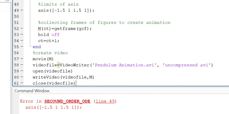
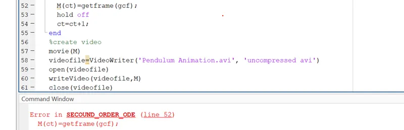
end

• I got two errors in the limit of the axis and collecting the frames. collecting frames are solved rewrite the 'M' Instead of 'm'
• another error is solved rewrite the line 49

RESULTS:

The plot is generated between the Angular displacement, angular velocity, and time

SIMPLE PENDULUM:

https://youtu.be/Simple pendulum