Week 3 - Solving second order ODEs

AIM:

1. To write a program to solve the 2nd order ODE in MATLAB.

2. To Simulate the motion of the simple pendulum.

DESCRIPTION:

In Engineering, ODE is used to describe the transient behaviour of the system. A simple example is the simple pendulum.

The following assumptions are made before deriving the ODE using Newton's 2nd law of motion

1. The mass of the rod connecting the bob is assumed zero.

2. The mass of the bob is point mass.

Using Newton's 2nd law of motion, the second order ordinary differential equaiton is derived considering the assumptions as follows:

ma = N + F(weight of the bob)

ma = N + mg

a = a(normal) + a(tangential)

ma(tangential) = -mgsin(θ) (cancelling m on both sides)

a(tangential) = -g.sin(θ)-------------------(1)

v = l.θ (θ is of 1st order)
a = l.θ (θ is of 2nd order)

l.θ(2nd order) = -g.sin(θ)

θ(2nd order) = -(g/l).sin(θ)

θ(2nd order)+(g/l).sin(θ) = 0 -------------------(2)

The equation (2) is the 2nd order ODE for a simple pendulum without damping effect.

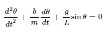
Considering Damping effect, the equation can be re written as :

-----------------(3)

MATLAB CODE DEFINITION:

The higher order differential equations has to be simplified or broken down into multiple lower order differential equation. The higher the order of ODE, higher the order of the matrix.

In this simple pendulum example, we have the highest order of 2. Hence, the order or maximum rows in the matrix will be 2.

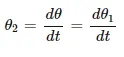
The 2nd order ODE is broken down into 1st order ODE'S by

--------------------(4)

--------------(5)

-------------(6)

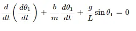
substituting (4) and (6) in (3) we get;

-----------(7)

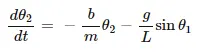
To solve the ODE, matlab requires the differential vairables to be in a matrix form and hence,

---------------------------------------(8)

--------------------------(9)

writing this in matrix form, w get

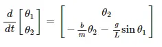-----------------------(10)

MATLAB CODE:

The input commands for the simple pendulum are mass of the bob (m), length of the pendulum, damping co-efficient (b) and acceleration due to gravity (g = 9.81 m/s2)

% simple pendulum

b = 0.05;
m = 1;
l = 1;
g = 9.81;

t_span = linspace(1,20,500);
theta_0 = [0;5];
[t,results] = ode45(@(t,theta) ODE(t,theta,b,g,l,m),t_span,theta_0);
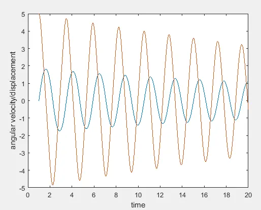
figure(1)
plot(t,results(:,1))
hold on
plot(t,results(:,2))
xlabel('time')
ylabel('angular velocity/displacement')

% simulating the motion of simple pendulum

ct = 1;
for i = 1:length(results(:,1))
    
figure(2)
x0 = 0;
y0 = 0;
x1 = l*sind(results(i,1));
y1 = -l*cosd(results(i,1));
plot([-0.08 0.08],[0 0],'linewidth',3,'color','b');
hold on;
line([x0 x1],[y0 y1],'linewidth',3);
plot(x1,y1,'o','markers',20,'markerfacecolor','r');
axis([-0.1 0.1 -2 2]);
title('Motion of the simple pendulum');
grid on;

pause(0.0003)

hold off

M(ct) = getframe(gcf)
ct = ct+1
end

movie(M)
videofile = VideoWriter('ode_func.avi','uncompressed avi')
open(videofile)
writeVideo(videofile,M)
close(videofile)

t_span = linspace(1,20,500)

This command assigns 500 values from 1 to 20 to the variable t_span

theta_o = [0;5]

This command assigns the 1st row(ang.displacement) as zero and 2nd row (ang.velocity) value as 5

[t,results] = ode45(@(t,theta) ODE(t,theta,b,g,l,m),t_span,theta_0)

This command ode45 integrates the equaiton (10) over the time span of 1 to 20 seconds with the initial condition of angular displacement 0 rad and angular velocity of 5 rad/s.

plot(t,results(:,1))

this command plots the x axis as t against the 1st column (ang displacement) of the 500x2 matrix of the result matrix

plot(t,results(:,2))

this command plots the x axis as t against the 2nd column (ang velocity) of the 500x2 matrix of the result matrix

for i = 1:length(results(:,1)

this command assigns the value of i from 1 to 500 as the results matrix has 500 rows and 2 columns.

x1 = l*cosd(results(i,1))

y1 = -l*sind(results(i,1))

these commands indicates the co-ordinate system of the bob.

To simulate the real time simple pendulum y1 is assigned negative value to get the plot in 2nd and 3rd quadrant where x value ranges from -infinity to +infinity and y value ranges from 0 to - infinity

plot(x1,y1,'o','markers',20,'markerfacecolor','r')

this command plots the x1 and y1 value as a marker of size 20 and face color as red

ERROR:

The second plot (time vs angular velocity alone)was displayed

SOLUTION:

while using multiple plot commands, hold on command should be used in between to seperate the 2 plots.

FUNCTION CODE DEFINITION:

% SIMPLE PENDULUM

function [dtheta_dt] = ODE(t,theta,b,g,l,m)
theta1 = theta(1)      % 1st row value
theta2 = theta(2)      % 2nd row value
dtheta1_dt = theta2
dtheta2_dt = ((-b/m)*(theta2))-(g/l)*sin(theta1)
dtheta_dt = [dtheta1_dt;dtheta2_dt]      % in matrix form
end

The function code definitions are explained above in the equations 4 to 8.

Google drive link:

MOTION OF SIMPLE PENDULUM