Week 3 - Solving second order ODEs

AIM - To write the program in Matlab that will simulate the simple pendulum motion.

GOVERNING EQUATION - The governing equation used in the program is the second-order differential equation which represents the equation of motion of a simple pendulum with damping.

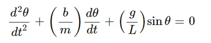
where,

b - Damping coefficient

m - The mass of ball in kg

g - Acceleration due to gravity (m/s2)

L - Length of the pendulum in m

so using the above equation I will show the animation of the simple pendulum for a fixed time span

OBJECTIVE - 1) To plot the variation of angular displacement and angular velocity with respect to the time of a simple pendulum.

2) To create the simple pendulum using the plot function and to animate it for the time span.

THEORY - A pendulum is a body suspended from a fixed support so that it swings freely back and forth under the influence of gravity. When a pendulum is displaced sideways from its resting, equilibrium position, it is subject to a restoring force due to gravity that will accelerate it back toward the equilibrium position. When released, the restoring force acting on the pendulum's mass causes it to oscillate about the equilibrium position, swinging it back and forth.

A simple pendulum is one that can be considered to be a point mass suspended from a string or rod of negligible mass. It is a resonant system with a single resonant frequency. The simple pendulum is shown below:

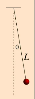
The period of a simple pendulum for small amplitudes θ is dependent only on the pendulum length and gravity. For the physical pendulum with distributed mass, the distance from the point of support to the center of mass is the determining "length" and the period is affected by the distribution of mass as expressed in the moment of inertia.

The image is shown below in which has the resolved trigonometric components.

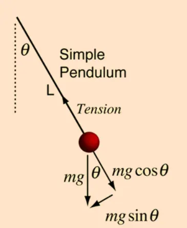
The equation of motion for the simple pendulum for sufficiently small amplitude has the form

ma = -mg`theta`

which when put in angular form becomes

`malphal = - mg(theta)` or `(d^2(theta))/(dt^2) + g/L*theta = 0`

This differential equation is like that for the simple harmonic oscillator and has the solution:

`theta = (theta)_max*sinsqrt(g/L)*t`

PROGRAM - The program to plot the time vs displacement and velocity and to simulate the simple pendulum is shown below:

% Program to simulate the pendulum motion
clear all
close all
clc
 % inputs
 l = 1;
 m = 1;
 b = 0.05;
 g = 9.81;
 
 % initial condition 
 % giving initial values for angular displacement and angular velocity
 theta_0 = [0;3];
 % giving the time span that will be from 0 to 20s
 t_span = linspace(0,20,400);
 
 % solving the ODE (calling the function)
 [t,results] = ode45(@(t,theta) ode_func(t,theta,b,g,l,m),t_span,theta_0);
 
% plotiing the time vs angular displacement and angular velocity
 plot(t,results(:,1),'color','r')
 hold on
 plot(t,results(:,2),'color','b')
 grid on
 xlabel('time');
 ylabel('Angular displacement and Angular velocity');
 legend(' Angular displacement','Angular velocity');
 
 
 % for animation of simple pendulum
 ct = 1;
 % using for loop so toget the whole time span
 for i = 1: length(t_span)
     x0 = 0;
     y0 = 0;
     x1 = l*sind(results(i,1));
     y1 = -l*cosd(results(i,1));
     
     figure(2)
     % plotting the origin or fix line of pendulum
     plot([-0.2 0.2], [0,0],'color','m','linewidth',2)
        hold on
     % plotting the length of the pendulum
     plot([x0 x1],[y0 y1],'linewidth',3,'color','b')
     % plotting the end point of the pendulum
     plot(x1,y1,'-o','markersize',10,'markerfacecolor','r')
     axis ([-0.5 0.5  -1.5 0.2])
     M(ct) = getframe(gcf);
     ct = ct + 1;
      hold off
 end
      movie(M)
    videofile = VideoWriter('simple_pendulum.avi','uncompressed AVI');
    open(videofile)
    writeVideo(videofile,M)
    close(videofile)
   

In the above program, the clear all command will delete the data from the previously performed operation, close all command will close all the graphs or scope related to the previously performed operation. clc command will clear the command window.

Then I have given the inputs for the length of the pendulum(l), the mass of the ball(m), damping coefficient(b), and the acceleration due to gravity(g). The values I have assigned are the input given to me.

Next, I have assigned the initial conditions that are at the time(t) = 0s the angular velocity is 3 and the angular displacement is also 0.

Then I know that the time span for which I have to calculate the results is 0 to 20s. so that is what I have written and also have used the linspace command to get multiple values of time between 0 to 20s.

Then for solving the differential equation I have called the function which I have created separately in another program. This function is like a template and can be used whenever required. The program for the function is shown below

function [dtheta_dt] = ode_func(t,theta,b,g,l,m)
theta1 = theta(1)
theta2 = theta(2)
dtheta1_dt = theta2;
dtheta2_dt = -(b/m)*theta2 - (g/l)*sin(theta1);
dtheta_dt = [dtheta1_dt;dtheta2_dt];
end
  

Here the ode_func is the name of the function and the inputs that I have to give to get the output from the function are (t that is time, theta that is displacement, damping coefficient(b), length(l), the mass of ball(m), and acceleration due to gravity(g)).

since the solver, I have to use is the ode45 and ode45(ode_fun,t_span,y_o), where tspan = [t0 tf], integrates the system of differential equations y′=f(t,y) from t0 to tf with initial conditions y0. Each row in the solution array y corresponds to a value returned in column vector t. This ode45 uses numeric integration to solve the equations. This solver will only able to solve one-degree equations so I have to convert the second-order equation into first order in order to get the results.

so in the above program, I have done exactly that. As we know that if theta is displacement so the differentiation of theta will give velocity. Here the governing equation will come:

if `theta = theta1`

then differentiating both sides

`(d(theta))/dt = (d(theta1))/dt = theta2`

again differentiating both sides

`(d^2(theta))/dt^2 = (d^2(theta1))/dt^2 = d/dt*(d(theta1))/dt = (d(theta2))/dt`

putting the values in governing equation

`(d(theta2))/dt + b/m(theta2) + g/Lsin(theta1) = 0`

so now it's converted and that I how I got the values:

`(d(theta))/dt = theta2 and (d(theta2))/dt = -b/mtheta2 - g/Lsin(theta1)`

and those are values that I have putten in the program. In the function, one column is for displacement and the other is for velocity. Then I have just ended the function.

Now going back to the main program as I have already mentioned about the solver that is ode45 I have also used the anonymous function in the same line. An anonymous function is a function that is not stored in a program file but is associated with a variable whose data type is a function handle. Anonymous functions can accept multiple inputs and return one output. They can contain only a single executable statement. so here the solver will two results one will be for angular displacement and the other will be for angular velocity.

Then I have plotted the time vs angular displacement and angular velocity and because I have to show both the outputs in one plot I have used the hold-on command. grid on will turn on the grids and legend will show which plot is what.

Then for simulating the simple pendulum I have to create the simple pendulum first and then simulate it.

so for that, I have used the 'for' loop command because I want to calculate results at different angles for the whole time span of 20 seconds. Then I have just defined the conditions that initially the pendulum will be stationary and after attaining some velocity which in my case is 3 it will displace. using the trigonometric functions I have found the equations for x1 and y1.

Then I have just plotted the simple pendulum which is my figure 2. I have created one fixed line from -0.2 to 0.2 on the x-axis and as I know that one end of the pendulum will be fixed at (0,0) and the other will be free.

Then I have plotted [x0 x1],[y0 y1] to get the length of the pendulum downwards in a negative y-direction and given the linewidth to increase the thickness of the line and assigned color to it as well.

Then I have plotted(x1, y1) to get the ball which will be at the end of the pendulum, and have used the marker size and marker face color command to get the circle shape of the required size and color. Then i have just fixed the range of x and y-axis using the axis command.

The get frame command will store each and every position of the pendulum and in that line, M is an array that will save the figure window. and the counter will increment by 1 on every next step.

Then I have simply ended the 'for' loop. we have to make sure that for each 'for' loop there is an end.

Then for the animation purpose since I have to show the simulation, I have to make the output in a video format. so for doing that I have used the movie command. so Matlab will create a video or say movie of the frames stored in the array (M). The video file is used to create the name and type of the video. The open and close command is used to open and close the video file. so here program to simulate the simple pendulum ends.

RESULTS - The output plot for time vs angular displacement and angular velocity is shown below:

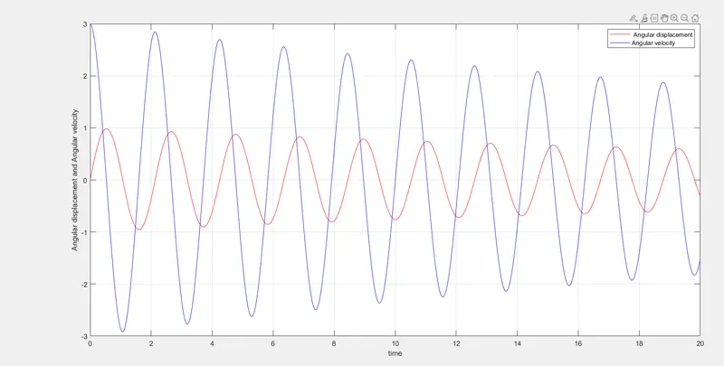
In the above fig., we can see that the angular displacement starts from 0 and the angular velocity starts from 3 rad/s which are my initial conditions, and then it shows the variation for the whole time span of 20 seconds.

The simulation of a simple pendulum can be seen using the link below:

https://drive.google.com/file/d/1ut8ZH4CKNoTJ0moY8qgcbTzrOtHa6BY_/view?usp=sharing

CONCLUSION - The program to plot Time vs Angular displacement and Angular velocity and to simulate the simple pendulum motion has been completed successfully and the results are shown.