Week 3 - Solving second order ODEs

SOLVING A SECOND ORDER ORDINARY DIFFERENTIAL EQUATION

OBJECTIVE:

To write a program to solve the second order differential equation of simple pendulum under oscillation to find the transient motion of the pendulum under different time periods.

INTRODUCTION:

• In this code, we are analyzing the motion of a simple pendulum which is oscillating under simple harmonic motion, with damper action.
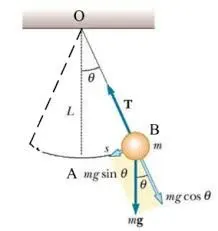
• A pendulum of length l is attached to the damper at one end, which is fixed (pivoted) and the other side of the pendulum is attached with a mass of m, the oscillation is carried out under gravity by an external stimulation.
• Our motive is to notice the positions of the pendulum under oscillation in different time periods.
• To help these things, the simple harmonic motion equation of a pendulum with a damper under oscillation ,

• 

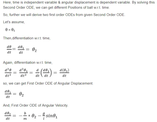
• In the above equation, in order to find the value of either velocity and acceleration, we need to find the value of theta by means of odeint solver which is an inbuilt solver in python under SciPy library.

• At first, we are creating a function named model where these differential equations are stored as an input. With some input parameters , which define these equations .

• After assigning the function , the integration carried out is an numerical integration , following the process of runge-kutta 4 th order numerical method will actually define these process.

• For numerical integration , we need to assign the initial condition and a time period to carry out .
• The solver odeint syntax is defined in similar way that it requires the function to be solved, initial condition and time periods and argument values that are predefined

The code for solving the second order differential equation is mentioned below ,

import math
import matplotlib.pyplot as plt 
import numpy as np
from scipy.integrate import odeint

#these are all the libraries we need to use in our program 

#this program is basically regarding the simple harmonic oscillation of the pendullum with damper action 
#now we are going to define the function named ode which stores the required validating equations and also it will return the values in the form of the differential 
#equation which is to be used on the upcoming steps and it will return the values in the form of the array 

def model(theta,t,b,l,g,m): # we are now creating a function where the equations are stored and processed for the required conditions 
	theta_1 = theta[0] #as we said the structure of the theta is displacement and velocity , for this line we need only displacement so calling the displacement value by index 0 
	theta_2 = theta[1]#we are now calling the velocity value by calling through the index value 
	dtheta_1 = theta_2 #after differentiation we are assigning the value accordingly 
	dtheta_2 = -(b/m)*theta_2-((g/l)*math.sin(theta_1)) #differentiating the ode and then replacing the value of it accordingly with the shm equation
	dtheta  = [dtheta_1,dtheta_2] #we are now storing the differential terms in a collective fashion as in the theta 
	return dtheta #these functions after processing the line by line it will return the output values in to the dtheta list or array 


#now we are assigning the variables or the arguments in the shm with damper equations
b = 0.05 #damping co-efficient 
g = 9.81 #acceleration due to gravity 
l = 1 #length of the pendullum 
m = 1 #mass of the pendullum

#as the odeint requires a initial condition to solve , the initial conditions are said to be 
theta_initial  = [math.radians(90),0]
#where the first value belongs to the displacement and the preceeding one belongs to the velocity accordingly , as per the calculation


#so we need to know the plots in a certain limits of time , this time-period is also essential one to the odeint solver 
t = np.linspace(0,20,150) #linspace is a parameter in the numpy array , which provides values according to the user defined value with the intervals , 
#here in this case the inputs are 0 and 10 the interval limits is specified by 150 


#inorder to solve the ode function we need to provide the inputs ,which are specified into it 
#the value of the theta is represented only by the means of integration , to obtain this we need to use the odeint solver here to get the values of the theta
#respectively

theta = odeint(model,theta_initial,t, args=(b,l,g,m))

#the syntax of the odeint solver is arranged accordingly in the above line , where it first requires the function to be solved, the initial value , the timeperiods
#and the arguments if necessary , in this case we predefined the arguments and the values are provided outside the function if suppose we need to change the values 
#it could be difficult if it is defined inside the fucntion 
#print(theta)
#print(theta_1)
#print(theta_2)
#now we are going to plot the values accordingly")
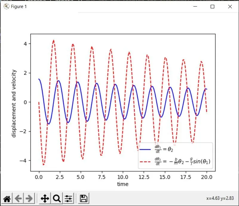
plt.plot(t,theta[:,0],'b-',label=r"$\frac{d\theta_1}{dt}=\theta_2$") #these line represnt the displacement of the pendullum and we are assigning a label to it 
plt.plot(t,theta[:,1],'r--',label=r"$\frac{d\theta_2}{dt}=-\frac{b}{m}\theta_2-\frac{g}{l}sin(\theta_1)$") #these line represents the velocity of the pendullum oscillation and assigning a label to it 
plt.xlabel("time") #we are now assigning a name to the x-axis
plt.ylabel("displacement and velocity ") #we are now assinging a name to the y-axis 

plt.legend(loc='best') #we are saying the solver to locate the legend in a best way accordingly 
plt.show() #this command is used to show the output of the plots

ct = 1      # we are creating a counter variable for saving the plots in an efficient way
T = theta[:,0]    #we are now calling only the displacement value for the pendullum oscillation 
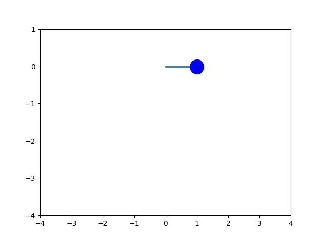
for THETA  in T:      #we are now implementing loop , for plotting the different positions of the pendullum with respect to time accordingly 
	x_0 = 0  #these are the origin point
	y_0 = 0 #these are the origin point
	x_1 = l*math.sin(THETA)  #this is nothing but the other end of the pendullum i n origin and in different positions .
	y_1 = -l*math.cos(THETA) #this is the other end of the pendullum , where the pendullum motion is along the y-axis .
	filename= 'text'+ str(ct) + '.png'   #we have created a variable called filename where the images are to be stored .
	plt.figure(ct)   #this will open a plot for certain condition in a new window 
	plt.plot([x_0,x_1],[y_0,y_1] , lw = "2") #now we have plotted the co-ordinates of the link1 , with some attributes
	plt.plot(x_1,y_1, marker = 'o', color = "blue", markersize=20)  #we are now assignning a attribute to other end of the pendullum 
	plt.xlim(-4,4) #now we have limited our graph to a definitive limits 
	plt.ylim(-4,1) #now we have limited our graph to a definitive limits
	plt.savefig(filename) #the opened window will be stored as an image in the location 
	ct = ct+1 #once after finish running the code for the initial image this command will append to the other element of the range provided.
	

CONCLUSION :

Thus the above code is implemented and can be used to find the displacement and velocity values of the simple pendulum under oscillation and can be used to plot it accordingly ,

from the above code we can also simulate a pendullum under oscillation .