Week 2 Air standard Cycle
OTTO CYCLE SIMULATOR USING ENGINE KINEMATICS IN PYTHON
Given below the program code that can solve the otto cycle and make plots for the thermal efficiency of an engine and generates a pv diagram of it taking in input values of :
- Bore diameter
- Stroke length
- Connecting rod length
- The compression ratio
- Start crank angle
- End crank angle
- The specific heat ratio or gamma
- The temperatures at intake and at combustion (power stroke )
Thermal efficiency for an otto cycle engine is given by the formula :
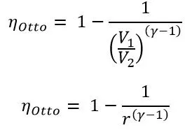
Where r is the compression ratio and gamma is the specific heat ratio
CODE :
|
# this program is to define the otto cycle with engine kinematics
thermal_efficiency = 1-(part1) print(thermal_efficiency) |
SOLUTION:
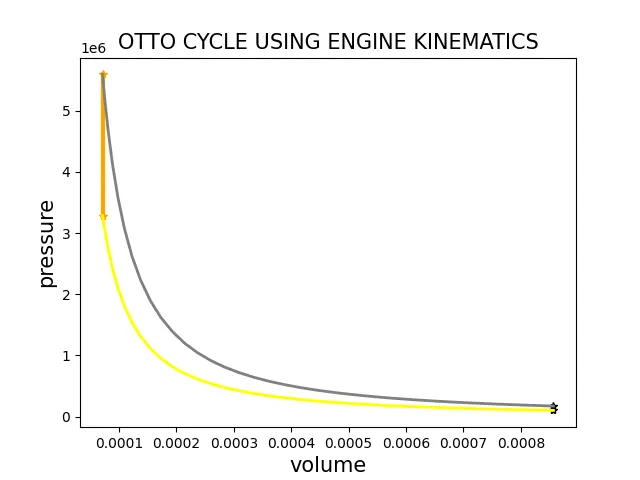
As we know for compression and expansion stroke , the piston is going to move in a linear motion where the pressure and volume will be fluctuating . whereas in the other state rather than the expansion and compression stroke , the volume is going to be same or constant . If we going to make a plot with these parameters obtained from all the 4 stages , the resulting graph wont appear accurately as the otto cycle , where the compression and expansion stroke volume and pressure will be produced as changing in a sequential manner , which is completely wrong . as the compression and expansion stroke will produce plots In a parabolic curves .in order to make the graph look pretty much similar to the actual graph , we need to import the engine kinematics which could possibily solve the problem , engine kinematics is nothing but the mechanism of the engine , which is mainly for the compression and expansion state . at first , we need to define the engine kinematics as function in the name of the engine kinematics , where the inputs are predefined for certain values. Engine mechanics is obviously based on the crank angles to . in order to define the engine kinematics with respect to the crank angles we are going to use a certain formula , where the volume of the cylinder is defined with certain parameters , which is to be defined manually and some parameters are actually predefined , this volume is for the movement of piston ,in actual terms this is the volume of the compression and expansion strokes , by using another formula ( adiabatic equation ) we could probably find the pressure for the compression and expansion stroke . the formulae are given below :
Engine kinematic – volume of the cylinder:
V = V_c*(1 + (1/2*(cr -1 ) * ( R + 1- cos(theta) * (R^2 – sin^2(theta))^0.5)
Adiabatic equations :
P*v^gamma = constant
By actually using these formula we can overcome the problem and can provide a realistic otto cycle graph . to find the crank angle we need to provide the constraints for the crank angle which are 0 and 180 degree for the piston at bottom dead centre and top dead centre respectively . by providing these constraints we are telling the program that we need the angles between this limit , that can we provided by an expression dtheta , which has the ending crank value and strating crank value which are defined accordingly for compression and expansion stroke , the dtheta is also a dependent of n_values , which means we are defining the program that we need these much no of values of crank and the volume of the compression and expansion accordingly . instead of defining the values of crank angle in a manual list we are creating a loop which could actually generate no of values in accordance with the range , which is provided manually by the user . the expression for the n_value is given below
dtheta = (ec – sc) /(n_values – 1) , this equation creates a value according to the n_values which is used for the loop to create a arithmetic sequential orders of the angle and the volume of the compression and expansion . here -1 is stated , because python always read the first value as 0 , if we provide 10 values the first value is actually 1 but to define for python we need to reduce that by compensating the equation by -1.
INPUTS WHICH ARE PREDEFINED :
- Bore = 0.1 m
- Stroke = 0.1 m
- Connecting rod = 0.15 m
- Compression ratio = 12 ( no units )
- Specific heat ratio = 1.4 ( no units )
- Temperature at intake (t1) = 500 in kelvins
- Temperature at power stroke ( t3) = 2300 in kelvins
Output graph :
# this program is to define the otto cycle with engine kinematics
import math
#we always import math module to perform certain mathematical calculations and formulations
import matplotlib.pyplot as plt
#for plotting the outputs we always require matplotlib and pyplot used to plot , which is called by its alias name plt
#geometric properties of the engine
bore = 0.1 #bore of the cylinder in m
stroke = 0.1 #stroke of the cylinder in m
con_rod = 0.15  #length of the connecting rod in m
cr = 12 #compression ratio of the thermal process


#now we are going to create a function , which has all the data of the engine
def engine_kinematics(bore,stroke,con_rod,cr,start_crank,end_crank) :
#as we have created a function named engine_kinematics which stores all the required information, and the values inside the set brackets are the inputs which can also be given manually
	a = stroke / 2
	R = con_rod / a
#this function consists of mechanism of the engine with respect to the different crank angles provided the  starting aand ending angle are the fixed inputs
	sc =  math.radians(0) #fixed input for the start angle of the crank
	ec =  math.radians(180) #fixed input for the  end angle of the crank
#as we said we are defining this function according to engine mechanics ,we are going to consider the entire volume of the engine using the formula
# V = V_c*(1+(1/2*(cr -1 )(R + 1-costheta)*(R^2 - sin^2(theta)^ 1/2))

	V_s = math.pi/4*pow(bore,2)*stroke  #this is the swept volume of the otto cycle during the intake of the process
	V_c = V_s / ( cr -1 ) #this is the clearance volume of the otto cycle or an engine during the compression process

	V = [] #we are creating a empty array , so that we could load the datas of volume of the engine generated with different values

	n_values = 50 #which is we are defining that the loop should provide 10 values of the theta

	d_theta = (ec - sc)/(n_values - 1) # this variable is called crank angle spacing and it is also a mathematical constant used for the loop which provides
#constant value according to the  n_values we provide , which is to be predefined

	for i in range(n_values): #we are defining the for loop with iterable variable with the range of n_values we provided
		 theta = sc + i*(d_theta) #the purpose of creating the loop is to provide the arithmetic sequence of values of the theta which is to be stored in the theta array

		 #now we are going to derive the equation for the cylinder volume of the engine in to a definitive  terms

		 term1 = 0.5*(cr-1)
		 term2 = R + 1 - math.cos(theta)
		 term3 = pow(R,2) - pow(math.sin(theta),2)
		 term3 = pow(term3,0.5) #here we have overwritten the variable to provide the necessary equation
		 #now we are going to define the volume of the cylinder of the engine
		 V.append(V_c*(1 + term1*(term2 - term3))) #we are using append parameter to say the program that it needs to be added in the memory  of the variable

	return V #the return statement is used to say the loop that once u finish one cycle of loop , having the value  that should be entered in the empty array
	#v and then start another cycle and repeat the same

#inputs given for the otto cycle of the engine kinematics

p1 = 101325 #pressure1 at the intake process of the otto cycle at pascals
t1 = 500   #temperature of the intake process of the otto cycle at kelvins
t3 = 2300 #temperature of the expansion process of the otto cycle at kelvins
gamma = 1.4  #it is the constant value used in iscentropic equations

#now we are going to interpret the values of the otto cycle at each state point respectively before that we are going to mention the volumes of the cylinder
# at state 1 - intake process

V_s = math.pi/4*pow(bore,2)*stroke  #this is the swept volume of the otto cycle during the intake of the process
V_c = V_s / ( cr -1 ) #this is the clearance volume of the otto cycle or an engine during the compression process
v1 =  V_s + V_c   #this is the total volume of tbe fuel intake process and it is also the volume of the state 1 process

#at state 2 - adiabatic compression

#by using the inputs obtained from the state1 we  could actually derive the necessary inputs required for the state 2 variables
#we know that at the compression stage the clearance volume will be equal to the volume at the compression stage that is v2

v2 = V_c
p2 = p1*pow(v1,gamma) / pow(v2,gamma) #using the equation p2v2^gamma = p1v1^gamma we could actually derive the value of p2
rhs = p1*v1 / t1
t2 =  p2*v2 / rhs #these two equations are derived actually from the ideal gas equation to get the necessary equation , p2v2/t2 = p1v1/t1
V_compression = engine_kinematics(bore,stroke,con_rod,cr,0,180) #this equation is to create the curve for the otto cycle at different volume and different pressure

#to define P_compression , using the adiabatic compression equation p.v^gamma = constant
constant = p1*pow(v1,gamma) #the constant value is derived from the respective state process equation
P_compression = []

for v in V_compression :
	P_compression.append(constant/pow(v,gamma))


#at state3 ,constant volume heat addition

#as the otto cycle is the constant volume process , therefore the volume of the heat addition process will be equal to v2
v3 = v2

rhs = p2*v2 / t2
p3 = rhs * t3 / v3 # actually we are using the same variable equation method as the previous state to acquire the respective equation


#at state 4  ,  iscentropic expansion

v4 = v1 #same volume as the volume of the intake volume as the piston moves to its original position after heat addition process
p4 =  p3*pow(v3, gamma) / pow(v4, gamma) #obtained using the equation p4v4^gamma = p3v3^gamma
t4 =  p4*v4 / rhs   #here no need to mention the rhs  again as it is going to consider the rhs as a constant value

#the same method has used in compression is used here for expansion
constant = p3*pow(v3,gamma)

V_expansion = engine_kinematics(bore,stroke,con_rod,cr,180,0)
P_expansion = []

for v in V_expansion:
	P_expansion.append(constant/pow(v,gamma))


font1= {'family': ' roman ','color':'black', 'size': ' 15'}
#now we are provided a dictionary , stored with keys and values of the data that has the requirements for the title and other labels


plt.plot([v2,v3],[p2,p3], marker ="*",color='orange',lw='3') #this represents the constant volume heat addition process
plt.plot([v4,v1],[p4,p1], marker ="*",color='black',lw='3') #this represents the constant volume heat rejection process
plt.plot(V_compression,P_compression,color='yellow',lw='2') #this represents the compression process
plt.plot(V_expansion,P_expansion,color='grey',lw='2')#this represents the expansion process

plt.title("OTTO CYCLE USING ENGINE KINEMATICS", font1) #alloting a relevant title for the process
plt.xlabel("volume",font1) #alloting a specific blabel to the graph
plt.ylabel("pressure",font1) #alloting a specific label to the graph
plt.show()


#and finally we are going to provide the thermal efficiency of the otto - cycle
part1 = 1 / pow(cr,gamma-1)
thermal_efficiency = 1-(part1)
print(thermal_efficiency)