Solving second order ODEs - Damping of an oscillating pendulum

A. OBJECTIVE:

1. To write a program in Matlab to Solve ODE representing the motion of a simple pendulum with damping.
2. To create a plot showing the damping.
3. To create an animation from the acquired output images.

B. TERMINOLOGIES:

Pendulum : body suspended from a fixed point so that it can swing back and forth under the influence of gravity.

Damping : is an influence within or upon an oscillatory system that has the effect of reducing or preventing its oscillation.

Damping of pendulum

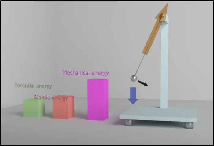
A pendulum undergoes simple harmonic motion if no external forces act on the pendulum. As a result the pendulum’s angular displacement is modeled as a function of time, assuming the pendulum retains its angular amplitude and starts its oscillation at its angular amplitude.

However if an external force acts on the pendulum, this model is not suitable because the pendulum will undergo damping. As a result, the pendulum’s angular amplitude decreases over time due to the total energy of the pendulum is being transferred to the surrounding environment. Eventually the pendulum will lose all of its energy and stop oscillating.

C. FORMULAS

Second order of this damping is defined by the equation :

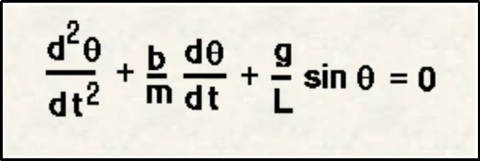
Where,

g = gravity in m/s^2

L = length of the pendulum in m

m = mass of the body in Kg

b = damping coefficient

For solving the above second degree order equation it has to be broken down to first degree,

θ1 = θ2

θ2 = -b/mθ2 -g/l sinθ1

D. PROGRAMMING IN MATLAB

close all
clear all
clc
 
%Known inputs
b = 0.05;
g = 9.81;
l = 1;
m = 1;
 
%for angular displacement = 0 and angularvelocity = 3rad/sec
theta_0=[0;3];
 
%time point- simulation between 0-20 seconds
time_span = linspace (0,20,300);
 
%solving ode
[t,results] = ode45(@(t,theta)ode_func(t,theta,b,g,l,m),time_span,theta_0);
 
figure(1);
plot(t,results(:,1),'linewidth',1); %diplacemnt 
hold on
plot(t,results(:,2),'linewidth',1); %angular velocity
xlabel('time');
ylabel('plot');
grid on
legend({'dsplacement','velocity'})
 
ct=1;
for i = 1:length(results(:,1))
    x=0;
    y=0;
    x1= l*sin(results(i,1));
    y1= -l*cos(results(i,1)); %motion of pendulum with respect to theta
    
    figure(2)
    plot([-2,2],[0,0],'linewidth',3,'color','b');
    line([x x1],[y y1],'linewidth',2,'color','r');
    hold on;
    
    plot(x1,y1,'o','markers',20,'markerfacecolor','g');
    grid on;
    axis([-3 3 -3 3]);
    pause(0.05);
   
    M(ct) = getframe(gcf); 
    ct = ct+1;
    
     hold off;
end
%creating movie
movie(M);
videofile = VideoWriter('pendulumanimate.avi','UNCOMPRESSED AVI');
open(videofile);
writeVideo(videofile,M);
close(videofile);

E. EXPLANATION

1. Clear all,close all,clc command is used to clear data stored in workspace,close plot and figures and clear the command window respectively.
2. Known inputs such as the damping coefficient(b),Length of the string(l),Mass of the suspended body (m) and the gravity value is given as inputs.
3. Theta value is defined starting from displacement as 0 and angular velocity at 3.
4. Time span is defined from 0 to 20 seconds with 300 values in between using the lindspace command.
5. Matlab can only accept a 1^stdegree ODE thus it is necessary to covert a 2^nd degree ODE to 1^st
6. Defining a function named ode_func.

   function [dtheta_dt] = ode_func(t,theta,b,g,l,m)
    
   theta1 = theta(1)
   theta2 = theta(2)
   dtheta1_dt = theta2;
   dtheta2_dt = -(b/m)*theta2 - (g/l)*sin(theta1);
   dtheta_dt = [dtheta1_dt; dtheta2_dt];
   end​

7. Using the inbuilt ODE45 function the value of displacement and angular velocity is calculated at each value of theta over a defined time period.
8. A for loop is initialized to capture the frame of the plot after each iteration.
9. An array M is created to store the image generated of the current frame using the ‘getframe(gcf)’ function.
10. The VideoWriter command creates a video file with the name ‘pendulumanimate and saves it in .avi format.
11. The writevideo command insert the frame stored in array M into the videofile.

F. RESULTS

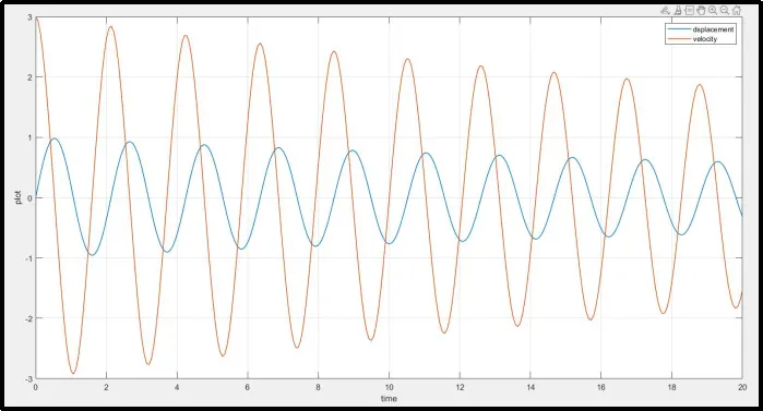
1. Figure 1

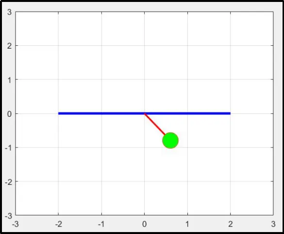
2. Figure 2

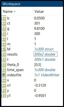
3. Workspace

4. Animation of the oscillating pendulum : Damping of Pendulum

G. ERRORS

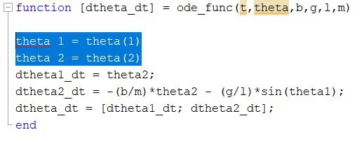
error 1 - Identifier Theta both a variable ad command

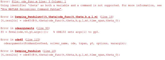
• Space between the theta and 1,2 respectively treated it as a variable and a command.

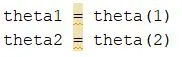
• It was solved by removing the space thus making theta 1 and 2 variables.

error 2 - Couldn't output the video file

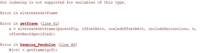
• error was raised due to calling the hold off command before iteration

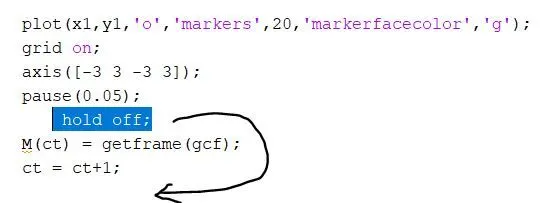
• it was solved by calling it after the iteration

 plot(x1,y1,'o','markers',20,'markerfacecolor','g');
    grid on;
    axis([-3 3 -3 3]);
    pause(0.05);
   
    M(ct) = getframe(gcf); 
    ct = ct+1;
    
     hold off;

H. CONCLUSION

1. Plot for angular velocity and displacement with respect to time was done. It was noted how with time the angular velocity reduced due to damping reducing the oscillation of the pendulum.
2. A movie file was made showing the animation of the oscillation