SLOVING SECOND ORDER DIFFERENTIAL EQUATION, USING PYTHON PROGRAMMING LANGUAGE

AIM:

• To solves the Ordinary Differential Equation using Python programming language.

OBJECTIVE:

• The main objective is to solve the differential equation given below, which represents the equation of motion of a simple pendulum with damping.

`frac{d^2theta}{dt^2} xx frac{b}{m} . frac{d theta}{dt} xxfrac{g}{l} sin theta =0`

In the above equation,

g = gravity in m/s2,

L = length of the pendulum in m,

m = mass of the ball in kg,

b=damping coefficient.

• Also other main objective is to animate the motion of the pendulum between 0-20 seconds

GOVERNING EQUATIONS:

• As the motion of the simple pendulum is a second order differential equation. This must be broken down into two First order differential equations,
  
  • `theta = theta1`
  • `frac{d theta}{dt} =frac{d (theta1)}{dt} = theta2`
  • `frac{d^2 theta} {dt^2} = frac {d}{dt} . frac{d (theta1)}{dt} = frac {d}{dt) . theta2`
  • `frac {d(theta2)}{dt} = - [ frac{b}{m} . theta2 xx frac{g}{l} sin theta1]`
• As per the above single order differential equations the motion of the simpule pendulum can be determined. As the following static inputs are given in the code,

Length of the pendulum, L=1 metre,

Mass of the ball, m=1 kg,

Damping coefficient, b=0.05.

Acceleration due to gravity, g=9.81 m/s2.

DETAILED CONTENT :

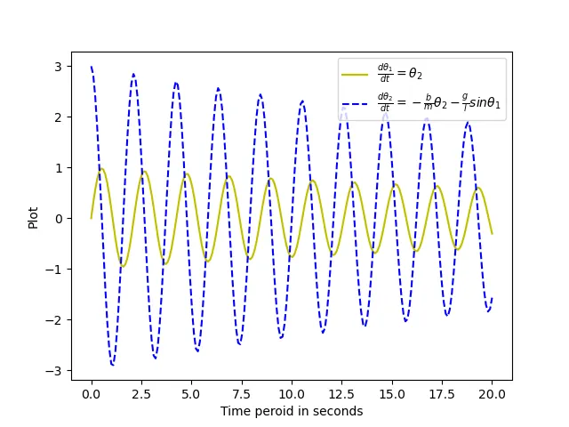
• Based of the given parameters and using ODEINT function, which is imported from scipy module. The two first order differential equation of simple pendulum can be sloved and the image of the angular displacement and Angular velocity with respect to time can be plotted.
• Note that, The two first differential equation's value computed using ODEINT is stored in the vector form only, Hece the values which are to be ploted should be called accordingly.
• The Motion of the simple pendulum is simulated between 0-20seconds. For the angular displacement 0 radians and the Angular velocity is 3 radian per second. Thus for each value of time, the image with respect to position of the pendulum is captured and those images are stitched together and then animated using image magick software.

PYTHON CODE WITH EXPLAINATION:

"""
TO SIMULATE THE MOTION OF SIMPLE PENDULUM
"""

#IMPORT THE MODULES /LIBRARY TO BE USED IN THE PROGRAM
import math
import matplotlib.pyplot as plt
import numpy as np
from scipy.integrate import odeint 



#DEFINING FUNCTION TO SLOVE FIRST ORDER DIFFERENTIAL EQUATIONS
def change_in_position (theta,t,b,m,g,l):
	# DEFINING THETA_1 AND THETA_2 IN A VECTOR FORM
	theta_1 = theta[0]
	theta_2 = theta[1]
	# AS THE SECOND ORDER DIFFERENTIAL EQUATION IS CONVERTED INTO THE TWO SINGLE ORDER DIFFERENTIAL EQUATION
	dtheta1_dt = theta_2
	dtheta2_dt = - ((b/m) * theta_2 )- (g/l) * math.sin(theta_1)
	# SAVING THE VALUES IN VECTOR FORM
	dtheta_dt = [dtheta1_dt, dtheta2_dt]
	#RETURN THE VALUES WHICH IS COMPUTED.
	return dtheta_dt


#INPUT PARAMETERS 

#length = 1 meter
l = 1
#Mass = 1 Kg
m = 1
#Damping Coefficient = 0.05 no units
b = 0.05
#Acceleration due to gravity = 9.81 m/s^2
g = 9.81

#INTIAL CONDITION 
theta_0 = [0 , 3]

#TIME VARIATIONS FROM 0 TO 20 SECONDS
t=np.linspace(0,20,200)

#CALLING THE FUNCTION, USING ODEINT IMPORTED FROM SCIPY MODULE 
theta = odeint (change_in_position,theta_0,t, args = (b,m,g,l))

#PLOT RESULTS
""" 
THE SOLUTION OF DIFFERENTIAL EQUATION CAN BE PLOTTED
THE ANGULAR DISPLACEMENT IN RADIAN PLOTED
THE ANGULAAR VELOCITY IN RAD/SEC CAN BE PLOTTED
"""
# TO PLOT THE ANGULAR DSPLACEMENT AND ANGULAR VELOCITY WITH RESPECT TO TIME 
plt.plot (t,theta[:,0],'y-',label= r'$frac{dtheta_1}{dt}=theta_2$')
plt.plot (t,theta[:,1], 'b--', label = r'$frac{dtheta_2}{dt}= - frac{b}{m}theta_2 - frac{g}{l}sintheta_1$')
#PLOTING THE X & Y LABELS
plt.xlabel ("Time peroid in seconds")
plt.ylabel("Plot")
# TO PLOT THE LEGENTS IN THE BEST LOCATION
plt.legend(loc ='best')
#TO SHOW THE PLOT
plt.show()

# TO PLOT THE MOTION OF SIMPLE PENDULUM, ANIMATION BASED ON THE POSITION OF PENDULUN, WTH RESPECT TO TIME  
#DECLERING THE VARIABLE,ct FOR SAVING THE FILE IN SEQUENCE MANNER 
ct =1
for t1 in theta[:,0]:
	x0 = 0
	y0 = 0
	#LENGTH OF PENDULUM AT X-AXIS, WITH RESPECT TO THETA 
	x1 = (l * math.sin(t1))
	# AS THE LENGTH OF PENSULUM IN Y-AXIS, WITH RESPECT TO THETA, IT MUST BE  -VE AXIS 
	y1 = - (l * math.cos(t1))
	#SAVING THE FILE NAME AND INCREMENTING THE VARIABLE ct FOR SAVING THE PLOTS IN THE SEQUENCE MANNER
	filename = str (ct)+'.png'
	ct = ct+1
	#COMMAND FOR OPENING EACH PLOT IN A NEW TAB/ WINDOW
	plt.figure()
	#PLOTTING THE BASE FOR THE PENDULUM, WHERE IT HANGS 
	plt.plot ([-1,1], [0,0], 'blue', linewidth = 3.5)
	#PLOTTING THE LENGTH OF THE PENDULUM	
	plt.plot ([x0,x1] , [y0,y1], linewidth = 1, color= 'y')
	#PLOTTING THE ORIGIN OF THE PENDULUM IN THE BASE WHERE IT HANGS
	plt.plot (x0,y0,'o',markersize = 5)
	#PLOTTING THE POSITION OF THE BALL AT THE END OF THE PENDULUM 
	plt. plot (x1,y1, 'o', markersize = 30, color = 'r')
	#PLOTTING THE IMAGE  LIMITS
	plt.xlim([-1.5,1.5])
	plt.ylim([-1.5,1.5])
	#TITLE OF THE PENDULUM
	plt.title ('Animation of Simple pendulum')
	#SAVING THE PLOTS FOR ANIMATION
	plt.savefig(filename)

OUTPUT AND RESULTS:

• The Plot of Angular displacement and angular velocity with respect to time is shown below

• The output displaced while generating 200 images, is shown below,

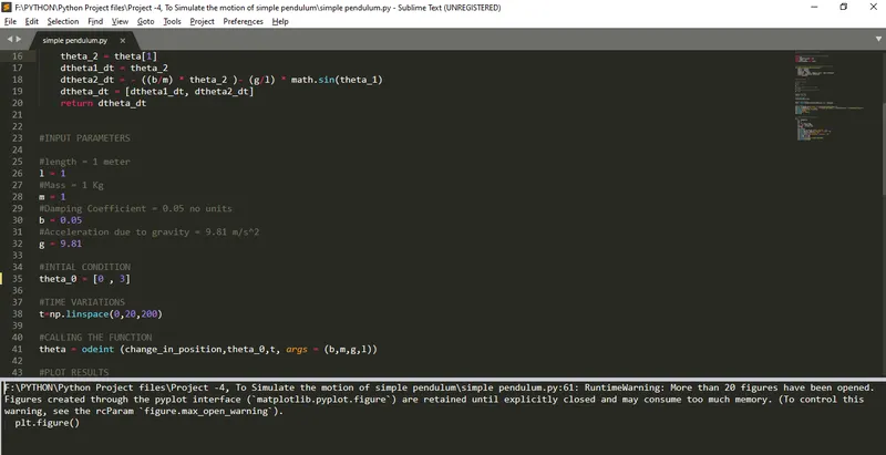
As this output is displaying warning massage, as many plots (200 plots) are being saved and this will comsume more memory.

• Using the link below, Animation of simple pendulum can be viewed,

https://drive.google.com/drive/folders/1SQ6W1aYjiznYOWAU5s4PhXLOX-LDFFyP?usp=sharing

CONCLUSION:

Hence, the transient behaviour of differential equations can be easily studied using Python program. One thing to note is that the higher order differential equation must be broken down into several first order equation and then only it be sloved using ODEINT function imported from the scipy module of PYTHON Programming language.