SOLVING AIR STANDARD CYCLE - OTTO CYCLE, USING PYTHON PROGRAMMING LANGUAGE

AIM:

• Write a program in python to solve OTTO CYCLE, with plotting P-V diagram.

OBJECTIVE:

• To Calculate the Efficiency of Otto cycle
• To plot P-V diagram of Otto cycle, Using engine Kinematics, to plot the volume covered by the piston for the different position of crank angle.

INTRODUCTION:

• The Otto Cycle, describes how heat engines turn gasoline into motion. Like other thermodynamic cycles, this cycle turns chemical energy into thermal energy and then into motion. The Otto cycle describes how internal combustion engines (that use gasoline) work.
• The Otto cycle, Has two Reversable adiabatic or Isentrpic process and two Isochoric process
• The otto Cycle, has following four process:
  • Process 1-2: Reversible adiabatic compression
  • Process2-3: Constant volume heat addition
  • Process 3-4: Reversible adiabatic expansion
  • Process 4-1: Constant volume heat rejection
• For Example we can take, Four Stroke Spark-Ignition Engine. In a four-stroke engine, the cycle of operations is completed in four strokes of the piston or two revolutions of the crankshaft.
• An ideal four-stroke SI engine consists of the following four strokes:
  • Suction or intake stroke
  • Compression stroke
  • Expansion or power stroke
  • Exhaust stroke
• In these four strokes, the four Otto cycle process is carried out based on the movement of the pistion inside the engine cylinder.
• Each stroke consists of 180° of crankshaft rotation and hence a four-stroke cycle is completed through 720° of crank rotation.

ASSUMPTIONS OF OTTO CYCLE:

• The working substance is air and it behaves as an ideal gas.
• The working substance has a fixed mass. (Closed System Analysis)
• The specific heats of working fluid do not change with temperature.
• The working fluid does not undergo any chemical change.
• All the processes are reversible processes

GOVERNING EQUATIONS:

• SWEPT VOLUME : `frac{Pi}{4} xx D^2 xx l`

Where, D - Is the dia of the engine cyclinder. L - is the depth of the engine cyclinder

• CLEARANCE VOLUME: swept volume x `frac{1}{r-1]`

Where, r - Is the compression ratio

• IDEAL GAS EQUATION: `P xx V^gamma` = Constant

Where, `gamma` - Is the adiabatic index

• EFFICIENCY OF OTTO CYCLE: `1 - frac{1}{r^(gamma-1)}`

DETAILED CONTENT:

• All the input parameters are assumed (Refer code), with that It’s easier to find the temperature and pressure at the each state and easier to calculate the efficiency of the otto cycle using the above equations.
• It is easier to generate the plot of the P-V diagram. But, the isentropic process will be also linearly plotted which is not acceptable. Hence for that the relation between the position of the crank (Crank angle) and the volume of the piston covered equation to be derived.
• Using Engine kinematics, the the relation between the position of the crank (Crank angle) and the volume of the piston covered, is given below

where, V = Volume covered ; Vc = Clearance Volume ; R = Length of connecting rod / crank radius; `theta`= crank angle or the position of the crank

• For Process, 1-2: Isentropic compression, For isentropic compression, The piston must move from BDC to TDC. The starting crank angle is 180 degree and the ending crank angle is 0 degrees, within which the crank angle varies and these angles are used in sequence for plotting the graph. Using the above relation, the volume of the piston covered at various position of crank can be determined. Thus, for different volumes at different position of the crank, corresponding pressure can be obtained using ideal gas equation. Hence, using the values, it is easier to plot which gives the correct parabolic path between state-1 and state-2.
• For Process, 2-3: Constant Volume heat addition, In this process the heat addition takes place, but the volume remains constant, pressure increases from p2 to p3 (Maximum pressure).
• For Process, 3-4: Isentropic expansion, For isentropic expansion, The piston must move from TDC to BDC. The starting crank angle is 0 degree and the ending crank angle is 180 degrees, within which the crank angle varies those values are used in sequence for plotting the graph. Using the above relation, the volume of the piston covered at various position of crank can be determined. Thus, for different volumes at different position of the crank, corresponding pressure can be obtained using ideal gas equation. Hence, using the values, it is easier to plot which gives the correct parabolic path between state-3 and state-4.
• For Process, 4-1: Constant Volume heat rejection, This process occurs during the exhaust stroke. process the heat is rejected. And the volume remains constant, pressure increases from p4 to p1 (Minimum pressure).

PYTHON CODE WITH PROPER EXPLAINATION:

"""
TO PLOT THE PV DIAGRAM OF OTTO CYCLE & TO CALCULATE THE EFFECIENCY OF THE ENGINE 
"""

#IMPORT THE MODULES / LIBRARY  WHICH ARE TO BE USED IN THE PROGRAM 
import math
import matplotlib.pyplot as plt 

#DEFINING A FUNCTION FOR INGINE KINAMATICS
"""
This function helps to get the relation between the Crank angle and the swept volume.
The main use of derving relation is used to plot the graph of Change in pressure and Change in Volume during the compression and the expansion stroke.
"""

def change_in_volume (length_cd, Radius_crank, r,v_c, theta_start, theta_end ):
	#The equation for change in volume with the crank angle is given below,
	"""
	V = {1+ ½ (r-1) [ 1+R – cos theta – (R^2 – sin^2 theta)^1/2]} v_c (Refer Report for the detailed Explaination)
	Where, R = length_cd / Radius_crank 
	"""
	volume_variation =[]
	theta_variation = []
	Num_values = 100
	for i in range (0,Num_values):
		#Each 10 degrees are ploted using dtheta 
		change_theta =theta_start + i * ((theta_end - theta_start) / 18)
		theta_variation.append(change_theta)


	for theta in theta_variation:
		R= length_cd / Radius_crank
		term_1 = 0.5 * (r-1)
		term_2 = 1+ R - math.cos (theta)
		term_3 = pow (R,2)
		term_4 = pow (math.sin (theta),2)
		term_5 = pow (term_3 - term_4, 0.5)
		vol = 1 + term_1*(term_2 - term_5)
		final_V= vol * v_c
		volume_variation.append (final_V)


	return (volume_variation)


# ENGINE PARAMETERS 

#Bore dia of the engine in meters
bore_dia = 0.5

#Length of the bore in meters
length_bore = 0.5

#The length of the connecting rod in meters
length_cd = 3

#Crank Radius in meters
Radius_crank = length_cd /2 

#Swept volume in m^3
v_s= (math.pi /4) * pow (bore_dia,2) * length_bore
#compression ratio of the otto cycle has no units 
r=10
#Clearence volume in m^3
v_c = v_s / (r-1)
#Adiabatic constant , gamma = 1.4 
gamma = 1.4
 
#Pressure at state-1 , P1 in bar; Temperature at state -2, T1 in kelvin
p1 = 1.01325
t1 = 500

#The Volume at state-2 and Volume in state -2 in m^3
v1 = v_s +v_c
v2 = v_c

#PROCESS -1 : Adiabatic compression 

"""
Using Ideal gas equation,  (p1 * v1^ gamma) = (p2 * v2^gamma)
To find Pressure at state p2 = (p1 * v1^ gamma) / v2^gama in bar
 """
p2 = (p1 * (pow (v1, gamma))) / (pow (v2, gamma))

""" 
To plot graph, in accurate manner the change in volume for change in theta to be calculated.
that is we need to plot the volume at the different change in the position of the crank angle.
calling the function for ploting the finding the volume change in the different angles of crank using compression stroke 
During compression stroke the piston moves from BDC TO TDC, the crank angle changes from 180 degrees to 0 degree
theta_start = 180 , theta_end = 0
"""
v_compression =change_in_volume (length_cd, Radius_crank, r,v_c, math.pi , 0)

# For the respective change in volume during compression the change in pressure os to be determined
# Using ideal gas equation , p v^gamma = constant
constant= p1 * pow (v1, gamma)
p_compression =[]
for q in v_compression:
	 change_pressure = constant / pow (q, gamma)
	 p_compression.append(change_pressure)

#PROCESS-2 : Isochoric process, Constant Volume heat addition

"""
(p1 * v1) /t1 = (p2 *v2) / t2

to find the temperature at state-2, t2 = (p2 *v2 * t1) / (p1 * v1) in kelvin
"""
t2 = (p2 *v2 * t1) / (p1 * v1)

"""	
(p3 * v3) /t3 = (p2 *v2) / t2
to find the temperature at state-4, t = (p2 *v2 * t1) / (p1 * v1)
The temperature after the combustion is assumed as 1800 K
"""
t3 = 1800
v3=v2
p3 =  (p2 * v2 * t3) / (t2 *v3)

#PROCESS -3: Adiabatic Eapansion
"""
Using Ideal gas equation,  p2 * v2^ gamma = p3 * v3^amma
To find Pressure at state p3 = (p2 * v2^ gamma) / v3^gamma
constant volume, v4=v1
"""
v4 = v1
p4 = (p3 * (pow (v3, gamma))) / (pow (v4, gamma))


""" 
To plot graph, in accurate manner the change in volume for change in theta to be calculated.
that is we need to plot the volume at the different change in the position of the crank angle.
calling the function for ploting the finding the volume change in the different angles of crank using expansion stroke 
During expansion stroke the piston moves from TDC TO BDC, the crank angle changes from 0 degrees to 180 degree
theta_start = 0 , theta_end = 180
"""
v_expansion =change_in_volume (length_cd, Radius_crank, r,v_c, 0, math.pi)
# For the respective change in volume during compression the change in pressure os to be determined
# Using ideal gas equation , p v^gamma = constant
constant1=p3 * pow (v3, gamma)
p_expansion =[]
for w in v_expansion:
	 change_pressure_1 = constant1/ pow (w, gamma)
	 p_expansion.append(change_pressure_1)

#PROCESS -4: Isochoric process, Constant Volume heat rejection
"""
(p3 * v3) /t3 = (p4 *v4) / t4
to find the temperature at state-4, t = (p2 *v2 * t1) / (p1 * v1)
"""

t4 = (p4 *v4 * t3) / (p3 * v3)


#To find the Efficiency of the OTTO cycle
e= 1 - (1 / (pow (r, gamma-1)))

print ("swept Volume, v_s = ", v_s, "m^3")
print ("Clearance volume, v_c = ", v_c, "m^3")
print ("compression ratio, r = ",r, "no units" )
print ("Adiabatic constant, gamma =", gamma, "no units")
print ("Pressure at state-1, p1 = ", p1, "bar")
print ("Pressure at state-2, p2 = ", p2, "bar")
print ("Pressure at state-3, p3 = ", p3, "bar")
print ("Pressure at state-4, p4 = ", p4, "bar")
print ("Volume at state-1, v1 = ", v1, "m^3")
print ("Volume at state-2, v2 = ", v2, "m^3")
print ("Volume at state-3, v3 = ", v3, "m^3")
print ("Volume at state-2, v4 = ", v4, "m^3")
print ("temperature at state-1, t1 = ", t1, "kelvin")
print ("temperature at state-1, t2 = ", t2, "kelvin")
print ("temperature at state-1, t3 = ", t3, "kelvin")
print ("temperature at state-1, t4 = ", t4, "kelvin")

#CALCULATING EFFIENCY OF THE OTTO CYCLE

print ("Efficiency of the OTTO cycle, E  = ", e, "no units")
print ("Efficiency of OTTO cycle in terms of percentage =", e*100, "%")

#PLOTTING PV- DIAGRAM:
plt.plot (v_compression,p_compression, label ='Process -1 to 2 :Isentropic compression')
plt.plot ([v2,v3] , [p2,p3], label ='Process -2 to 3 :Isochoric heat addition')
plt.plot (v_expansion,p_expansion, label ='Process -3 to 4 :Isentropic expansion')
plt.plot ([v4,v1],[p4,p1], label ='Process -4 to 1 :Isochoric heat rejection')
plt.xlabel ("volume in cubic meters")
plt.ylabel ("Pressure in Bar")
plt.title ("PV Diagram for OTTO cycle")
plt.savefig("PV Diagram for OTTO cycle,Output")
plt.legend()
plt.show()

OUTPUT AND THE RESULT:

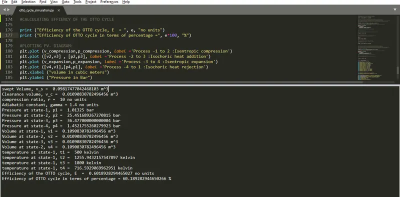
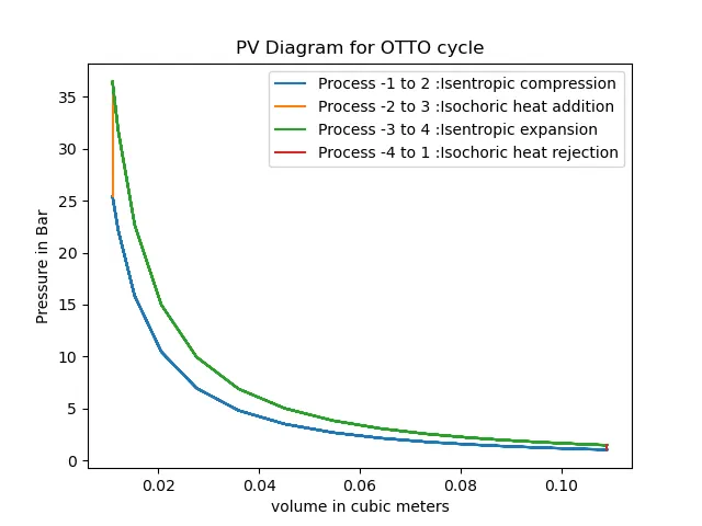
CONCLUSION:

• Hence, For the given input parameters, the Otto cycle effecieny can be easily calculated using python program and its PV diagram can be ploted.