DETAILED STUDY ON THE BEHAVIOR OF DRAG FORCE EXPERIENCED BY A CYCLIST, USING PYTHON PROGRAMMING LANGUAGE

AIM:

To study the behavior of the drag force experienced by a cyclist while moving certain distance. This study is done by two cases such as,

CASE-1: Calculating drag force against a cyclist by varying the flow Velocities and assuming other parameters constant.

CASE-2: Calculating drag force against a cyclist by varying the position of riding (Different shapes) having same frontial area but varying Drag-coefficient and assuming other parameters constant.

OBJECTIVE:

- Using Python Program, to calculate drag force.

- Using Python program to plot a graph, Velocity vs Drag force

- Using Python program to plot a graph, Drag Co-efficient vs Drag force

GOVERNING EQUATION :

DRAG FORCE : It is the resistive force, which is caused by the motion of the cyclist through flow air. It is a force which acts opposite to the direction of the oncoming flow velocity. This is the relative velocity between the cyclist and the flow air. The drag force D exerted on a cyclist traveling though the flowing air is given by,

Drag force, D =`frac{1}{2}xxrhoxxc_d xx A xx v^2`

where,

`rho` - Density of the flowing air in `(kg)/m^3`

`c_d` - Drag Coefficient (No Units)

A - Frontial area in `m^2`

V - Flow Velocity in `m/s`

DETAILED CONTENT:

CASE -1 : Writing a Python program, For calculating drag force against a cyclist by the below inputs. And also to plot graph (Velocity vs Drag force) for studing the effect of velocity on the drag force.

DENSITY : According to the international standard of atmosphere, Density of air 15 degree Celsius, is stated as 1.225`(kg)/m^3`

FORNTAL AREA : Frontal area has also the significant effect on the drag force. As it is directly proportional to the drag force, Hence, the frontal area increases the drag force increases linerly, and vice versa. Here we assume the frontal Area of the cyclist as 2`m^2`.

DRAG COEFFICIENT : It is the Dimensionless number, that relates objects drag force to its area and speed. Assuming the Drag coefficient as 0.8

FLOW VELOCITY: It is the relative velocity between the cyclist and the flow air. This is assuming twenty five inputs between (4.2 `m/s` to 12.5 `m/s`)

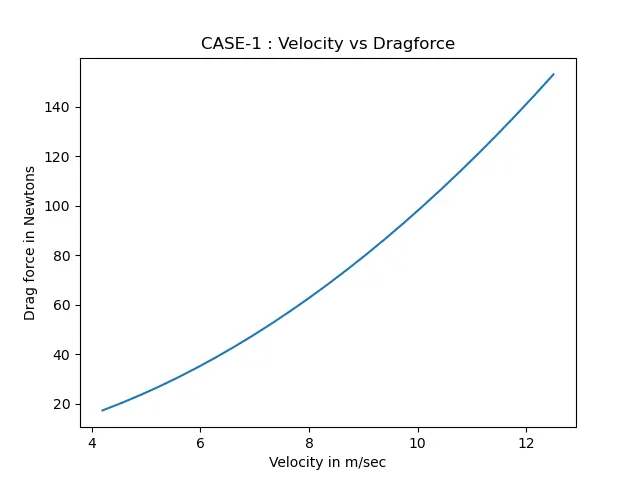
Thus, Using the above inputs, CASE-1 program will be exexuted and the plot (Velocity vs Drag force) is obtained, Which is used to learn the effect of Flow velocities on the Dragforce.

CASE -2 : Writting a Python program, For calculating drag force against a cyclist by the below inputs. And also to plot graph (Drag coefficient vs Drag force) for studing the effect of drag coefficient on the drag force.

DENSITY : According to the international standard of atmosphere, Density of air 15 degree Celsius, is stated as 1.225`(kg)/m^3`

FORNTAL AREA : Frontal area has also the significant effect on the drag force. It is directly proportional to the drag force, As the frontal area increases the drag force increases linerly, and vice versa. Here we assume the frontal Area of the cyclist as 2`m^2`.

DRAG COEFFICIENT : It is the Dimensionless number, that relates objects drag force to its area and speed. The shape of objects has very great amount on the affect of drag. Here the input for Drag coefficients are assumed 0.295, 0.45, 0.70, 1.28, 1.14. These values are taken from NASA's website published by Glenn research center.

For same Frontal area , the Drag coefficient changes for different shapes such as

Drag coefficient for bullet shape is 0.2950

Drag coefficient for Airfoil shape is 0.45

Drag coefficient for sphere shape is 0.70

Drag coefficient for Flat plate is 1.28

Drag coefficient for Prism is 1.14

FLOW VELOCITY: It is the relative velocity between the cyclist and the flow air. Flow velocity is assumed as 12.5 `m/s`

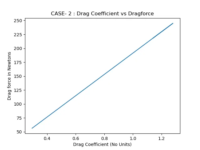
Thus, Using the above inputs, CASE-2 program will be exexuted and the plot Drag Coefficient vs Drag force is obtained, Which is used to learn the effect of Drag coefficient on the Dragforce.

PYTHON CODE FOR BOTH CASE-1 & CASE-2:

#CASE-1 :Plot Velocity vs Dragforce (Drag force against a cyclist)
"""
Assuming Twenty five Varying velocities(V) in m/s, And Keeping the other following parameters constant such as,
- Forntial area (A), in m^2
- Density of wind (D), in kg/m^3
- Drag Coefficient (C_D)  No units
Using above parameters the Twenty five different Drag force (D_F) in Newton, can be calculated.
And The graph against (velocity vs dragforce) will be plotted
"""
import math
import matplotlib.pyplot as plt
import numpy as np

#defining a Funtion for the input Velocity
def velocities (input_velocity):
	#Assinging an Empty array for obtaing Drag force output
	Drag_force=[]
	for i in input_velocity:
		#Input for Forntial area (A), in m^2
		A=2
		#Input for Density of wind (D), in kg/m^3
		D=1.225
		#Input for Drag Coefficient (C_D)  No units
		C_D = 0.8
		#Calculating Drag force
		D_F = (0.5*A*D*C_D*i * i)
		Drag_force.append(D_F)

	return (Drag_force)

#Main program
#Calling the function by giving the input to Velocities function
#input velocity, 25 inputs taken between (4.2 m/s to 12.5 m/s)

input_velocity = np.linspace(4.2,12.5,25)
result_1= velocities (input_velocity)
print ('CASE-1 : VALUE OF DRAG FORCE FOR DIFFERENT INPUT VELOCITIES')
print (result_1)
plt.figure(1)
plt.plot (input_velocity,result_1)
plt.xlabel('Velocity in m/sec')
plt.ylabel('Drag force in Newtons')
plt.title('CASE-1 : Velocity vs Dragforce')
plt.savefig('Velocity vs Dragforce')
plt.show()




#CASE-2: Plot Drag Coefficient vs Dragforce (Drag force against a cyclist)
"""
With Five Varying Drag Coefficient and Keeping the other following parameters constant such as,
- Forntial area (A), in m^2
- Density of wind (D), in kg/m^3
- Velocity (V) in m/s
Using above parameters the five different Drag force (D_F),Can be calculated. 
And The graph against (Drag Coefficient vs dragforce) will be plotted
"""

def Drag_Coefficient(input_C_D):
	#Assinging an Empty array for obtaing Drag force output
	Drag_force=[]
	for i in input_C_D:
		#Input for Forntial area (A), in m^2
		A=2
		#Input for Density of wind (D), in kg/m^3
		D=1.225
		#Input for Flow Velocity (V), in m/s
		V = 12.5
		#Calculating Drag force
		D_F = (0.5*A*D*i*V * V)
		Drag_force.append(D_F)

	return (Drag_force)
"""
Main program
Calling the function by giving the input to function
Drag Coefficient for the same frontial area is given as an Input but for different shapes 
Inputs For same frontal area the Drag Coefficient Varies for different shapes
C_D for bullet shape is 0.2950
C_D for Airfoil shape is 0.45
C_D for sphere shape is 0.70
C_D for Flat plate is 1.28
C_D for Prism is 1.14

"""
input_C_D = [0.295,0.45,0.7,1.28,1.14]
result_2= Drag_Coefficient (input_C_D)
print ('CASE-2 : VALUE OF DRAG FORCE FOR DIFFERENT DRAG COEFFICIENT')
print (result_2)
plt.figure(2)
plt.plot (input_C_D,result_2)
plt.xlabel('Drag Coefficient (No Units)')
plt.ylabel('Drag force in Newtons')
plt.title('CASE- 2 : Drag Coefficient vs Dragforce')
plt.savefig('Drag Coefficient vs Dragforce')
plt.show()

OUTPUT AND RESULTS:

DRAG FORCE OBTAINED FOR CASE-1 & CASE-2:

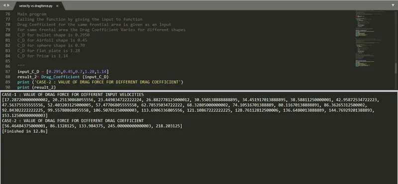
RESULT FOR CASE-1 :

RESULT FOR CASE-2:

CONCLUSION:

CASE-1: Velocity Vs Drag Force:

- As per the graph plot (Velocity vs Drag force), We can conclude that the curve is non liner and it is showing the parabolic curve.

- Drag force is directly perpendicular to the squared velocity, the most important point to note is Drag force increases rapidly with increase in flow velocity.

- Hence, I’ll conclude by stating “When Flow velocity is minimum, the Cyclist can achieve the maximum speed with less drag force”.

CASE-2: Velocity Vs Drag Force:

- As per the graph plot (Drag coefficient vs Drag force), We can conclude that the curve is liner.

- Thus the drag force changes linearly with the drag coefficient, It is important for a cyclist to minimize the drag coefficient for experiencing minimum drag force.

- Hence, I’ll conclude by stating “For same frontal area, if the position is adjusted for minimum drag Coefficient, The Cyclist can achieve a maximum speed with experiencing minimum drag force”.