FINAL INDEPENDENT PROJECT
Aim: Simulation of water reservoir system using MATLAB.
Objective:
1. The objective of Water Reservoir Simulation is to calculate all the important variables which affect the performance of the water reservoir system. The simulation should follow these conditions:
Conditions:
While simulating this system, the following assumptions are made:
- Simulation is done for 60 consecutive months.
- Water received through direct Rain Fall is assumed to be not more than 30% of the capacity of the reservoir.
- Maximum water received through River Inflow is not more than 130% of the capacity of the reservoir.
- Seepage loss is not more than 5%.
- Evaporation loss is not more than 8%.
- The water demand is never more than the Capacity of the Reservoir.
2. Print the variables (VI, VPM, GV, SL, EL, TL, VNET, DEMAND, SHORTAGE, SPILL, MONTHS) in the command window.
3. Plot the graph between:
- Plot the graph of the variations in Net Volume and Demand over the months.
- Plot the graph of the variations in Shortage and Spill over the months.
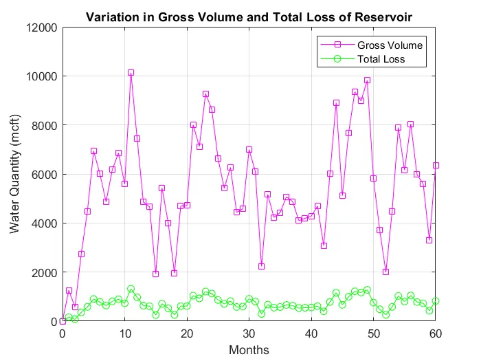
- Plot the graph of the variations in Total Loss and Gross Volume over the months.
The motivation of this project:
The motivation of this project was to forecast the reserve estimation of the water reservoir. This simulation will help to study the future scenario of the water reservoir.
Theory:
The increasing water demand for economic development, on the one hand, and the necessity of environmental control including water control, on the other, makes the problem of water management one of the most urgent tasks today. To solve this problem, it is essential to develop large-scale water resources systems. The term “water resource systems” comprises water sources, means of their control, and transportation to water users. Though the water resource system has many common features with all large–scale national economic systems, they differ from them to some extent due to a number of peculiarities. One of them, variability of river runoff, causes the stochastic character of process connected with the selection of parameters of water resources systems and their operational rules. Water consumption is also stochastic. This is determined by fluctuations of peculiarities, the process of soil formation.
Moreover, other unknown or uncertain factors of a technical and economic character may also be of considerable importance. Therefore, to solve the problem of water supply to the national economy, one must analyze the problem of coordination between stochastic water resources and the demand in them.
Reservoir simulation is a widely used tool for making decisions on the development of new fields, the location of infill wells, and the implementation of enhanced recovery projects. It is the focal point of an integrated effort of geosciences, petrophysics, reservoir, production and facilities engineering, computer science, and economics.
- Storage is necessary to regulate highly variable water flows. Reservoir for more constant uses such as municipal and industrial water supply, irrigation, hydroelectric power generation, and navigation.
- Typically, the water drawn from a reservoir is used at a much slower (and constant) rate than the rate and consistency of the water flowing into the reservoir
- Reservoir modeling has typically been employed to help size reservoir storage capacities, establishing operating policies, evaluating operating plans, administering water allocations, developing management strategies, and real-time operations.
- The term “Reservoir System Operations” refers to the practice of maintaining and managing a reservoir for multiple purposes, under dynamic conditions.
- The word “system” is used because of the complexity inherent in the operations of a typical reservoir or network of reservoirs.
- The state of the reservoir system is constantly in flux, requiring dynamic methods of simulation to evaluate and model them.
- The term “Reservoir System Operations Model” refers to a computer program used for simulating and optimizing changes in storage, water deliveries, and flood control for one or multiple reservoirs.
- Oftentimes, the objective of the reservoir operation is to balance the control of flood storage and maintain a reliable water supply.
- Operational procedures are different for flood events than what is employed under water-scarce conditions and therefore, the model must be adapted for these changing conditions.
- To better manage potential changes to reservoir operations given uncertainties or changes in circumstances, it is helpful to develop a calibrated simulation model of the reservoir.
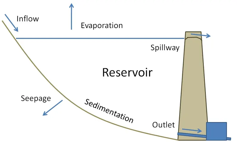
Fig: Water Reservoir System
Abbreviation and Terms used:
- M= Months
- C= Capacity
- RF= Rainfall
- RI=River Inflow
- VI= Volume Inflow
- VPM= Volume of Previous Month
- GV= Gross Volume
- SL= Seepage Loss
- EL= Evaporative Loss
- TL= Total Loss
- V_NET= Net Volume
- Demand
- Shortage
- Spill
MATLAB Code:
%Program for simulation of water reservoir system using MATLAB.
clear all;
close all;
clc;

VPM(1) = 0;                      % The initial value of VPM is assumed 0;
M=60;                            % Simulation run (in months)
C=input('Enter the capacity of reservior(in Million Cubic Feet): ');    % To request user input

% To make header of the output data
Header1=('\n Months  Volume Inflow   Volume of     Gross Volume   Seepage Loss   Evap. Loss     Total Loss     Net Volume       Demand       Shortage        Spill \n');
Header2=('                       Prev. Month \n');

% To print header in output
fprintf(Header1)
fprintf(Header2)

warning('off')      %To ignore this warning: Ignoring extra legend entries.

% Loop and Conditions

for i=2:M+1

    Months(i)=i-1;

    r1=rand;            % To generate random number-1 for rainfall
    r2=rand;            % To generate random number-2 for river inflow
    r3=rand;            % To generate random number-3 for demand

    RF(i)=r1*C*0.3;             % Condition for rainfall
    RI(i)=r2*C*1.3;             % Condition for river inflow
    VI(i)=RF(i)+RI(i);          % Condition for volume inflow

    GV(i)=VI(i)+VPM(i-1);       % Condition for gross volume of water

    SL(i)= GV(i)*0.05;          % Condition for seepage loss
    EL(i)= GV(i)*0.08;          % Condition for evaporative loss
    TL(i)= SL(i)+EL(i);         % Condition for total loss of water from reservoir

    V_Net(i)= GV(i)- TL(i);            % Net volume
    Demand(i)= r3*C;                   % Demand of water by consumers

    if Demand(i) > V_Net(i)
        Shortage(i)= Demand(i)-V_Net(i);
        VPM(i)=0;
        Spill(i)= 0;
    else
        Difference(i)= V_Net(i)-Demand(i);

        if Difference(i) > C
            Spill(i)= Difference(i)-C;
            VPM(i)=C;
            Shortage(i)=0;
        else
            VPM(i)= Difference(i);
            Spill(i)= 0;
            Shortage(i)=0;
        end
    end
    % End of the conditions

    % To print all the data in output
    fprintf(' %d',Months(i))
    fprintf('       %08.2f',VI(i))
    fprintf('       %08.2f',VPM(i))
    fprintf('       %08.2f',GV(i))
    fprintf('       %08.2f',SL(i))
    fprintf('       %08.2f',EL(i))
    fprintf('       %08.2f',TL(i))
    fprintf('       %08.2f',V_Net(i))
    fprintf('       %08.2f',Demand(i))
    fprintf('       %08.2f',Shortage(i))
    fprintf('       %08.2f \n',Spill(i))

    %Plotting Figures
    figure(1)                                       % Create figure window-1
    plot(Months, Demand,'color','k', 'marker','o')   % To plot demand graph vs month
    plot(Months, V_Net,'color','b', 'marker','s')    % To plot net volume graph vs month
    hold on                                         % To retains plots in the current axes
    xlabel('Months')                                % Labelling x-axis
    ylabel('Water Quantity (mcft)')                 % Labelling y-axis
    title('Variation in Demand and Net Volume of Reservoir')    % To specify title of the figure
    legend('Net Volume','Demand')                   % Add legend to axes
    grid on                                         % To show the grids in plot


    figure(2)                                       % Create figure window-2
    plot(Months, Spill,'color','b','marker','o')     % To plot spill graph vs month
    plot(Months, Shortage,'color','r','marker','s')  % To plot shortage graph vs month
    hold on                                         % To retains plots in the current axes
    xlabel('Months')                                % Labelling x-axis
    ylabel('Water Quantity (mcft)')                 % Labelling y-axis
    title('Variation in Shortage and Spill of Reservoir')       % To specify title of the figure
    legend('Shortage','Spill')                      % Add legend to axes
    grid on                                         % To show the grids in plot


    figure(3)                                       % Create figure window-3
    plot(Months, TL,'color','g','marker','o')        % To plot total loss graph vs month
    plot(Months, GV,'color','m','marker','s')        % To plot gross volume graph vs month
    hold on                                         % To retains plots in the current axes
    xlabel('Months')                                % Labelling x-axis
    ylabel('Water Quantity (mcft)')                 % Labelling y-axis
    title('Variation in Gross Volume and Total Loss of Reservoir')     % To specify title of the figure
    legend('Gross Volume','Total Loss')             % Add legend to axes
    grid on                                         % To show the grids in plot

end     % End of the loop

%End of the program
Code Explanation:
- Firstly, clear all, close all, and clc commands were used to clear the workspace, close all the current open windows, and clean the command window, respectively.
- The initial value of VPM was assumed to zero [VPM(1)=0].
- The total month of simulation run is stored in variable “M” and after that input, the syntax is written to take the input of capacity of the reservoir.
- Print the header of the data.
- Now, a syntax is written to ignore the warning.
- Now from here, our loop starts. The loop will run from 2 to M+1. where "M" is months (simulation run). The value of M is already provided at the starting of the program.
- After that, the value of "i"' is stored in the variable "Months(i)".
- Now three random numbers are generated. These random numbers will be generated between 0 and 1 for every iteration run. These random numbers will be different in each iteration.
- Rainfall, River inflow, and Volume inflow are calculated. According to conditions, the amount of rainfall cannot be higher than 30% of the capacity of the reservoir and the water received from the river inflow cannot be more than 130% of the capacity of the reservoir. As we know that the amount of water received from rainfall and river inflow is random. So here I used random numbers for both cases. The random number is multiplied with the capacity of the reservoir and after that, I calculate their 30% (rainfall) and 130% (river inflow) to get value for the amount water received from rainfall and river inflow respectively.
Rainfall= random No. * Capacity of reservoir * 0.3
River Inflow= random No. * Capacity of reservoir * 1.3
- After that, I sum up both rainfall and river inflow amounts to calculate volume inflow.
Volume Inflow= Rainfall + River Inflow
- After next, to calculate the gross volume I have to add the volume inflow and the reservoir volume of the previous month. By adding these two we will get the gross volume of water. Initially, it was considered that the VPM for the first iteration is zero.
Gross Volume= Volume inflow + Volume of water in the previous month
12. Now it’s time to consider the water loss. Here I have taken two parameters in water loss i.e. Seepage Loss and Evaporative Loss. As per condition, I have assumed that seepage loss will be 5% of gross volume and evaporative loss will be 8% of gross volume. This will be the maximum amount of water loss from both.
Seepage Loss= Gross volume * 0.05
Evaporative Loss= Gross volume * 0.08
13. By adding seepage and evaporative loss be will get the value of the total loss of water from the reservoir.
Total Loss= Seepage loss + Evaporative Loss
14. At final, the net volume of water will be:
Net Volume= Gross volume – Total loss
- After that, by using random number 3 (r3) we will calculate the demand of water from the reservoir. Demand is also a random factor that why the random number is used here.
Demand= Random No. * Capacity of reservoir
- If the demand of water is more than the net volume, then there will be a shortage of water. If there is a shortage, then the water for next month (VPM) will be 0 and the spill will be also zero.
if Demand > Net Volume
then Shortage= Demand - Net Volume
VPM = 0
Spill = 0
- If the above statement is not true or say if demand is lower than the net volume then we have to calculate the difference between them.
Difference = Net Volume - Demand
- If the difference is lower than the capacity, which means we have extra water. That extra water needs to be spill because we can’t store them. Now we will follow these statements:
if Difference > Capacity of Reservoir
then
Spill = Difference - Capacity of Reservoir
VPM = Capacity of Reservoir
Shortage =0
else
VPM = Difference
Spill = 0
Shortage =0
- At this point, our loop and all conditions were ended. After that will we print all the variables in the output.
- Now we will plot the graphs of variations in variables. Here I plot three figures:
- Graph of the variations in Net Volume and Demand over the months.
- Graph of the variations in Shortage and Spill over the months.
- Graph of the variations in Total Loss and Gross Volume over the months.
- After plotting the graphs, I provided the labeling, title, and legends for all three plots.
- Now the program is ended.
Output (Command Window):
Enter the capacity of reservior(in Million Cubic Feet): 4200

 Months  Volume Inflow   Volume of     Gross Volume   Seepage Loss   Evap. Loss     Total Loss     Net Volume       Demand       Shortage        Spill
                       Prev. Month
 1       01257.10       00000.00       01257.10       00062.86       00100.57       00163.42       01093.68       02461.59       01367.91       00000.00
 2       00573.02       00000.00       00573.02       00028.65       00045.84       00074.49       00498.53       03170.72       02672.19       00000.00
 3       02721.43       00000.00       02721.43       00136.07       00217.71       00353.79       02367.64       02888.74       00521.10       00000.00
 4       04473.04       02233.78       04473.04       00223.65       00357.84       00581.50       03891.55       01657.77       00000.00       00000.00
 5       04705.20       04179.23       06938.98       00346.95       00555.12       00902.07       06036.91       01857.68       00000.00       00000.00
 6       01831.15       03446.93       06010.38       00300.52       00480.83       00781.35       05229.03       01782.10       00000.00       00000.00
 7       01416.45       00779.92       04863.39       00243.17       00389.07       00632.24       04231.15       03451.23       00000.00       00000.00
 8       05388.93       03723.93       06168.85       00308.44       00493.51       00801.95       05366.90       01642.97       00000.00       00000.00
 9       03135.57       02572.00       06859.49       00342.97       00548.76       00891.73       05967.76       03395.76       00000.00       00000.00
 10       03011.98       03950.78       05583.98       00279.20       00446.72       00725.92       04858.06       00907.28       00000.00       00000.00
 11       06179.11       04200.00       10129.89       00506.49       00810.39       01316.89       08813.01       01375.77       00000.00       03237.23
 12       03240.79       02972.79       07440.79       00372.04       00595.26       00967.30       06473.49       03500.70       00000.00       00000.00
 13       01881.96       00603.31       04854.75       00242.74       00388.38       00631.12       04223.63       03620.32       00000.00       00000.00
 14       04055.99       00339.62       04659.31       00232.97       00372.74       00605.71       04053.60       03713.98       00000.00       00000.00
 15       01585.86       00835.74       01925.48       00096.27       00154.04       00250.31       01675.16       00839.42       00000.00       00000.00
 16       04600.70       01262.25       05436.44       00271.82       00434.91       00706.74       04729.70       03467.45       00000.00       00000.00
 17       02734.50       01234.10       03996.74       00199.84       00319.74       00519.58       03477.17       02243.07       00000.00       00000.00
 18       00723.25       01130.46       01957.35       00097.87       00156.59       00254.46       01702.89       00572.43       00000.00       00000.00
 19       03558.77       03282.85       04689.23       00234.46       00375.14       00609.60       04079.63       00796.78       00000.00       00000.00
 20       01429.65       03868.98       04712.50       00235.62       00377.00       00612.62       04099.87       00230.89       00000.00       00000.00
 21       04132.55       03056.98       08001.53       00400.08       00640.12       01040.20       06961.33       03904.36       00000.00       00000.00
 22       04059.84       02766.96       07116.82       00355.84       00569.35       00925.19       06191.63       03424.67       00000.00       00000.00
 23       06507.01       04200.00       09273.98       00463.70       00741.92       01205.62       08068.36       00002.19       00000.00       03866.17
 24       04435.07       03354.72       08635.07       00431.75       00690.81       01122.56       07512.51       04157.79       00000.00       00000.00
 25       03283.07       02409.22       06637.79       00331.89       00531.02       00862.91       05774.88       03365.66       00000.00       00000.00
 26       03006.68       00928.25       05415.89       00270.79       00433.27       00704.07       04711.83       03783.58       00000.00       00000.00
 27       05338.75       02350.00       06266.99       00313.35       00501.36       00814.71       05452.28       03102.29       00000.00       00000.00
 28       02085.51       01059.95       04435.51       00221.78       00354.84       00576.62       03858.89       02798.95       00000.00       00000.00
 29       03522.93       01211.13       04582.87       00229.14       00366.63       00595.77       03987.10       02775.97       00000.00       00000.00
 30       05782.99       01959.22       06994.13       00349.71       00559.53       00909.24       06084.89       04125.67       00000.00       00000.00
 31       04143.67       01410.60       06102.89       00305.14       00488.23       00793.38       05309.52       03898.91       00000.00       00000.00
 32       00823.64       01436.18       02234.24       00111.71       00178.74       00290.45       01943.79       00507.61       00000.00       00000.00
 33       03731.27       00947.29       05167.45       00258.37       00413.40       00671.77       04495.69       03548.39       00000.00       00000.00
 34       03279.36       01031.68       04226.65       00211.33       00338.13       00549.46       03677.19       02645.51       00000.00       00000.00
 35       03396.64       02330.51       04428.32       00221.42       00354.27       00575.68       03852.64       01522.13       00000.00       00000.00
 36       02735.46       03598.85       05065.97       00253.30       00405.28       00658.58       04407.40       00808.54       00000.00       00000.00
 37       01277.08       03626.70       04875.94       00243.80       00390.08       00633.87       04242.07       00615.36       00000.00       00000.00
 38       00471.11       00897.27       04097.82       00204.89       00327.83       00532.72       03565.10       02667.83       00000.00       00000.00
 39       03295.89       00728.36       04193.16       00209.66       00335.45       00545.11       03648.05       02919.68       00000.00       00000.00
 40       03554.36       01856.20       04282.72       00214.14       00342.62       00556.75       03725.97       01869.77       00000.00       00000.00
 41       02833.51       00497.45       04689.71       00234.49       00375.18       00609.66       04080.04       03582.59       00000.00       00000.00
 42       02576.96       01799.20       03074.41       00153.72       00245.95       00399.67       02674.73       00875.54       00000.00       00000.00
 43       04207.98       03474.72       06007.17       00300.36       00480.57       00780.93       05226.24       01751.52       00000.00       00000.00
 44       05435.24       04200.00       08909.96       00445.50       00712.80       01158.30       07751.67       00344.70       00000.00       03206.97
 45       00908.74       03745.47       05108.74       00255.44       00408.70       00664.14       04444.60       00699.13       00000.00       00000.00
 46       03914.86       04200.00       07660.33       00383.02       00612.83       00995.84       06664.49       00218.73       00000.00       02245.76
 47       05151.81       04200.00       09351.81       00467.59       00748.14       01215.73       08136.07       03098.93       00000.00       00837.14
 48       04777.90       03886.27       08977.90       00448.89       00718.23       01167.13       07810.77       03924.50       00000.00       00000.00
 49       05930.15       04200.00       09816.42       00490.82       00785.31       01276.13       08540.28       03299.35       00000.00       01040.93
 50       01616.56       03386.34       05816.56       00290.83       00465.33       00756.15       05060.41       01674.08       00000.00       00000.00
 51       00337.41       00000.00       03723.75       00186.19       00297.90       00484.09       03239.66       03944.40       00704.74       00000.00
 52       01993.26       00335.80       01993.26       00099.66       00159.46       00259.12       01734.14       01398.33       00000.00       00000.00
 53       04127.67       03777.26       04463.47       00223.17       00357.08       00580.25       03883.22       00105.96       00000.00       00000.00
 54       04113.50       03277.74       07890.76       00394.54       00631.26       01025.80       06864.96       03587.22       00000.00       00000.00
 55       02873.63       04200.00       06151.38       00307.57       00492.11       00799.68       05351.70       00227.81       00000.00       00923.89
 56       03842.09       04200.00       08042.09       00402.10       00643.37       01045.47       06996.62       01389.48       00000.00       01407.13
 57       01777.22       01048.83       05977.22       00298.86       00478.18       00777.04       05200.18       04151.36       00000.00       00000.00
 58       04540.15       00664.54       05588.97       00279.45       00447.12       00726.57       04862.41       04197.86       00000.00       00000.00
 59       02625.98       00910.43       03290.52       00164.53       00263.24       00427.77       02862.76       01952.33       00000.00       00000.00
 60       05429.98       04200.00       06340.41       00317.02       00507.23       00824.25       05516.16       00420.93       00000.00       00895.23
>>
Output (Plots):
Figure-1
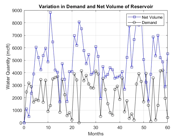
Figure-2
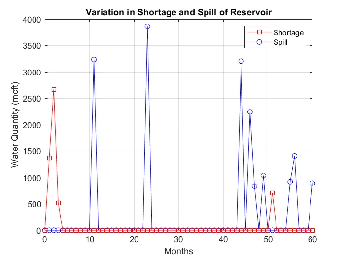
Figure-3
Conclusions:
- All three objectives were completed successfully.
- The MATLAB program follows all the initial conditions and boundary conditions.
- All three plots were generated and attached in the answer box.
- Output generated and provided in the answer box.
- After the simulation, the output data is validated by manual calculations to check it satisfies the conditions or not. it was found that the code is 100% accurate.
Future Scope:
The future scope of this project is to that we can go in deeper in this simulation by adding more boundary conditions such as soil type, soil condition, temperature, humidity, monsoon conditions, etc. By adding these boundary conditions, the accuracy of the simulation can be increased.