Week 3 - Solving second order ODEs

AIM: To simulate a simple pendulum motion using MATLAB program.

Simple pendulum is a string of axes connected to a bob at the free end of the axes, where the top end is fixed. The movement of the pendulum is based on newton's second law of motion. The suspended axes is completely based on the angular displacement, gravitational force and negative effect of the mass.

F=ma, where the acceleration is directly propotional to the force and inversely proptional to the mass of the pendulum.

using ODE45 function here to reduce any 4 to 5 ode functions to simple order functions by reducing it to single order differential equations into two sets to simulate the motion of the simple pendulum.

The formula relates with the:

• damping coefficient which is the resistant medium with respect to velocity, b
• angular displacement of the axes of the pendulum when subjected to free motion, theta1
• angular acceleration of the pendulum in free motion, theta2
• time to be noted for respective seconds, t
• gravitational force acting on the pendulum, g
• length of the pendulum, l
• mass of the bob, m

THE MAIN PROGRAM TO SIMULATE THE SIIMPLE PENDULUM MOTION:

clear all
close all
clc

%input values

b=0.05;          %damping coefficient
g=9.81;          %gravity
l=1;             %length of the pendulum
m=0.1;           %mass of the ball

%initial condition

theta_0=[0;3];

%timepoints

t_span=linspace(0,20,200);

%solve ODE
[t,results] = ode45(@(t,theta) ode_func(t,theta,b,g,l,m),t_span,theta_0);

%plotting results 1 and 2 with time graph
figure(1)
plot(t,results(:,1))        %time vs displacement
hold on
plot(t,results(:,2))        %time vs angular velocity
hold on
xlabel('time')
ylabel('angular displacement and angular velocity')
legend('angular displacement','angular velocity')
grid on

%for creating movie clip of pendulum
ct=1
for i=1:length(t)
    
    %coordinates
    x0=0;
    y0=0;
    
    x1=l*sin(results(i,1));
    y1=-l*cos(results(i,1));
    
    %for creating figure of pendulum
    %to create a beam
    figure(2)
    plot([-0.5 0.5],[0 0],'linewidth',4,'color','m');
    hold on
     
    %to create a string which connects beam to the sphere
    line([x0 x1],[y0 y1],'linewidth',2,'color','y');
    
    %to create sphere 
    plot(x1,y1,'O','markersize',15,'markerfacecolor','m');
    
    %to create a fixed axis
    axis([-1 1 -1 1])
    pause(0.3)
    hold off
    
    %to create animation
    
    M(ct) = getframe(gcf);
    ct = ct+1;
end

%to create and save the movieclip animated
movie(M);
videofile= VideoWriter('pendulum.avi','uncompressed AVI');
open(videofile)
writeVideo(videofile,M)
close(videofile)

THE ODE FUNCTION OF SEPERATED SINGLE ODE INSERTED TO THE MAIN PROGRAM:

function [dtheta_dt]=ode_func(t, theta, b, g, l, m)
theta1=theta(1)
theta2=theta(2)
dtheta1_dt = theta2;
dtheta2_dt=-(b/m)*theta2-(g/l)*sin(theta1);
dtheta_dt=[dtheta1_dt;dtheta2_dt];
end

EXPLANATION:

• start the program with clear all, close all, clc command to clear and stop any reccuring previous programs.
• start by giving input values of damping coefficient, mass of the bob, length of the pendulum, gravitational force, required time span.
• for the initial condition give the value for initial displacement and angular velocity.
• the linspace takes random values between 0 to 20 sec for required values.
• to enter ODE command for getting t and theta values, also ode function is inserted here which is already done in a new script where all values for the terms is noted.
• now to use plot command to plot displacement and angular velocity with time.
• hold on command used here to jump to next command without affecting the previous one.
• then label the graph with xlabel and ylabel command with respective names.
• using legend here to show the plot clear for undestanding.
• now to create a movie clip use contour command and for loop for representing the overall command for plotting figure 2.
• giving the starting and ending coordinates for creating the simple pendulum.
• then to use plot command for plotting fixed beam and string axes, with respected color and linewidth.
• then use marker command to create a sphere with respected points.
• use pause command for fixed time intervals while animating.
• use movie command to create animation of the simple pendulum with videofile name and close the command by giving close videofile.
• thus an animated clip will save in the drive.

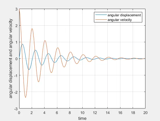
OUTPUT GRAPH:

THE ANIMATED CLIP LINK FOR SIMPLE PENDULUM:

https://drive.google.com/file/d/1LtWm66RG4P5fIR8SUX1hiS_meFohWNVt/view?usp=sharing

Thus, from the undestanding of the graph and animation we can say that the angular displacement and angular acceleration decreases with increase in time.