Week 3 - Solving second order ODEs

In Engineering, ODE is used to describe the transient behavior of a system. A simple example is a pendulum

The way the pendulum moves depends on the Newtons second law. When this law is written down, we get a second order Ordinary Differential Equation that describes the position of the "ball" w.r.t time.

Similarly, there are hundreds of ODEs that describe key phenomena and if you have the ability to solve these equations then you will be able to simulate any of theses systems.

Your objective is to write a program that solves the following ODE. This ODE represents the equation of motion of a simple pendulum with damping

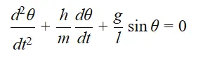
In the above equation,

g = gravity in m/s2,

L = length of the pendulum in m,

m = mass of the ball in kg,

b=damping coefficient.

Write a program in Python that will simulate the pendulum motion, just like the one shown in the start of this challenge.

use,

L=1 metre,

m=1 kg,

b=0.2.

g=9.81 m/s2.

Simulate the motion between 0-20 sec, for angular displacement=0,angular velocity=3 rad/sec at time t=0.

When you do this you will get the position of the pendulum as a function of time. Use this information to animate the motion of the pendulum

• For each value in time
• Create an image that represents the position of the pendulum
• You can assume the length of the string and the size of the ball
• Use the marker command to create a sphere
• One end of the pendulum is fixed
• The other end moves according to the solution of the ODE you had solved.
• If you are using using Matlab, use the movie command create an animation
• If you are using Octave you need to generate images first and then stitch them to form the animation

2. Submit a report that has the following content:

• Step wise explanation of your code.
• Errors faced while programming.
• How have you overcome those errors.
• Screenshots showing errors thrown in command window.

The presentation of your code will be taken into consideration while grading. Labelling sections of your code using comments is appreciated.

Upload the code using "INSERT SAMPLE CODE" option and then post screenshot of the plots generated.

In case if you are not able to finish the challenge, upload until what you have done and explain the procedure and plot. Deserved marks will be allotted.

Ans:

Solving a second order differential equation

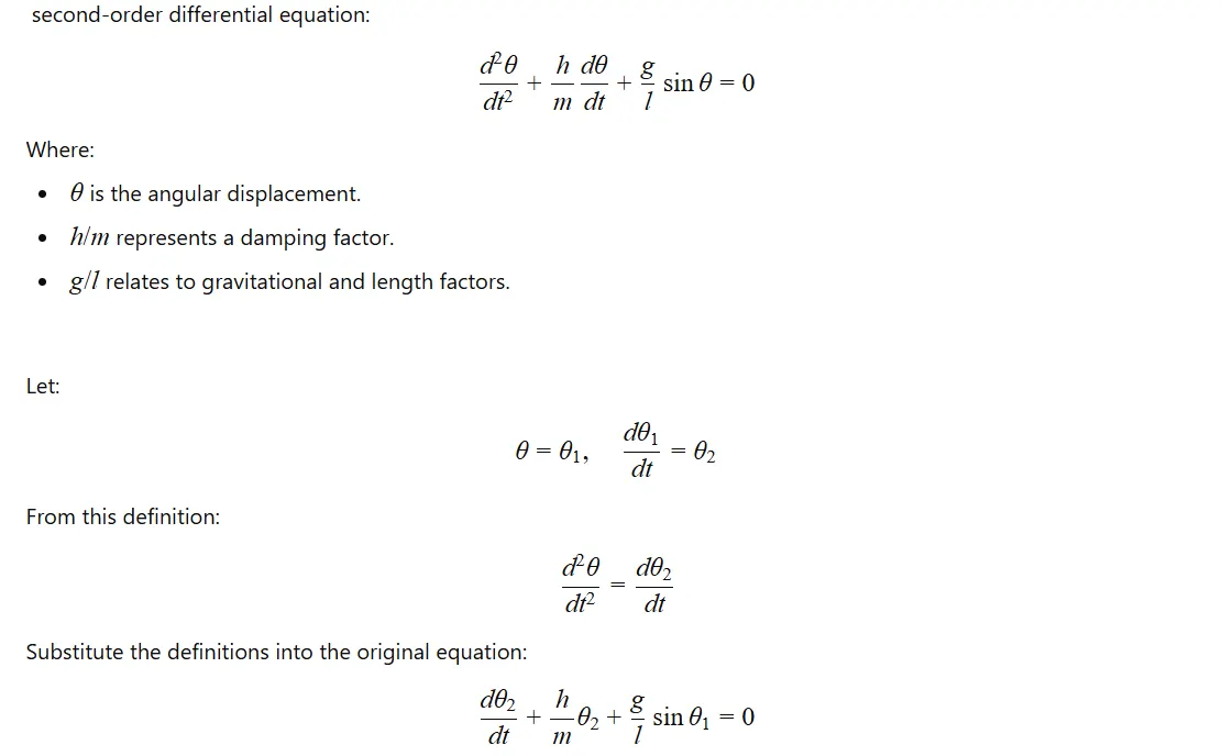
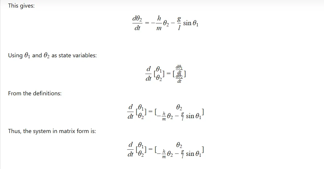
This sytem in matrix form we are using to get the response as well creating the simple pendulum.

Python Programs:

1) Plotting of simple pendulum

import numpy as np

from scipy.integrate import odeint

import matplotlib.pyplot as plt

from PIL import Image

# Function that returns d(theta)/dt

def model(theta, t, b, g, L):

theta1 = theta[0] # Angular displacement

theta2 = theta[1] # Angular velocity

dtheta1_dt = theta2

dtheta2_dt = -(b / m) * theta2 - (g / L) * np.sin(theta1)

return [dtheta1_dt, dtheta2_dt]

# Parameters

b = 0.2 # Damping coefficient

g = 9.81 # Gravity (m/s^2)

L = 1.0 # Length of the pendulum (m)

m = 1.0 # Mass of the pendulum (kg)

# Initial conditions

theta_0 = [0, 3] # Initial angular displacement (0 rad) and angula r velocity (3 rad/s)

# Time points

t = np.linspace(0, 20, 300) # Simulate from 0 to 20 seconds with 300 time points

# Solve ODE

theta = odeint(model, theta_0, t, args=(b, g, L))

angular_displacement = theta[:, 0] # Extract angular displacement

# Convert angular displacement to pendulum coordinates

x = L * np.sin(angular_displacement) # Horizontal position

y = -L * np.cos(angular_displacement) # Vertical position

ct=0

# Create and save images

for i in range(len(t)):

# Create a figure for each frame

filename=str(ct)+'.png'

ct=ct+1

fig, ax = plt.subplots(figsize=(6, 6))

ax.set_xlim(-1.2 * L, 1.2 * L)

ax.set_ylim(-1.2 * L, 1.2 * L)

ax.set_aspect('equal', adjustable='box')

# Plot pendulum

ax.plot((-0.2,0.2),(0,0),lw=10) # fixed base

ax.plot([0, x[i]], [0, y[i]], '-', lw=2, ) #pendulum

ax.scatter(x[i], y[i], color='blue', s=500,) #Bob

ax.text(-1, 1, f'Time: {t[i]:.2f} s', fontsize=12)

ax.legend()

# Save figure as image

plt.savefig(filename)

plt.show()

Here we find the theta 1 and theta 2 values and then also converting the angular displacement values to pendulum co-ordinates.

Then we create the plot of the pendulum. Here we fix the ais first so we are getting an even plot. and then we are plotting the base of hanging, pendulum and bob separeately. For bob we are using scattered plot as normal plot does not give the pendulum bob shape which we require.

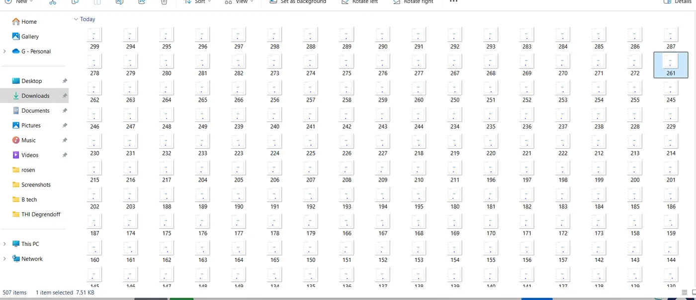
Images are generated and they are saved separately to the folder

2) Animation of simple pendulum

from PIL import Image

# Folder containing images

image_folder = r"C:\\Users\\sivap\\Downloads\\Pendulum images"

# List of image file paths

images = [f"{'Pendulum images'}\\{i}.png" for i in range(299)]

# Open all images and store them in a list

frames = [Image.open(img) for img in images]

# Save frames as an animated GIF

output_gif = "Pendulum_animation.gif"

frames[0].save(

output_gif,

save_all=True,

append_images=frames[1:], # Add the remaining frames

duration=100, # Duration for each frame in milliseconds

loop=0 # Infinite loop

)

We have taken individual images and stitched it together to form a an animation of the entire frames.

Output:

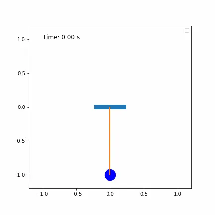
We can see that we have successfully created an animation of simple pendulum and we can observe that since we have given a damping coefficient of 0.2, the system starts to slowly damp after a few seconds.