Week 3 - Solving second order ODEs

Aim:

Write a python code to simulate the transient behavior of a simple pendulum and to create an animation of its motion.

Theory:

• In engineering, an ODE is used to describe the transient behaviour of a system. A simple example is a pendulum.
• Newton's second law determines the movement of a pendulum. When this law is written down, we get a second order Ordinary Differential Equation which describes the position of the 'ball' w.r.t time.

F = ma

• Here, the position(theta) of the bob w.r.t time is determined by using the second-order ODE which is

where, b= damping coefficient

g= gravity in m/s^2

m= mass of the ball in Kg

L= length of the pendulum in m

• In order to solve the second-order ODE, we convert it into a number of first-order ODEs. We will then create a separate function where we will assume two variables; theta1 and theta2.
• theta2 will be the first-order differential of theta1 and theat2= theta. Now, by using the equation given we will make a new relation for theta2, where theta2=-b/m*theta-g/l*sin(theta1).

Procedure:

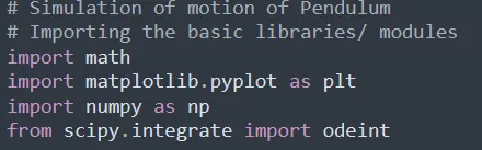
1. Import the modules.

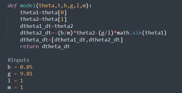
2. Define parmeters and input given parameters.

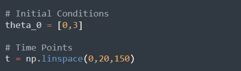
3. Define initial condition and time points (Initial time, Final time and no. of images).

4. Calculate the ODE.

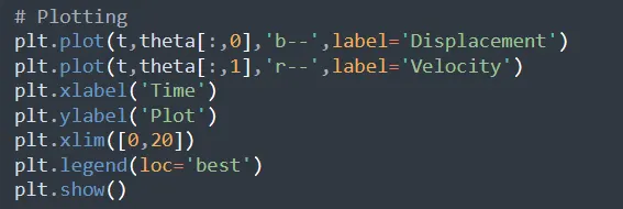
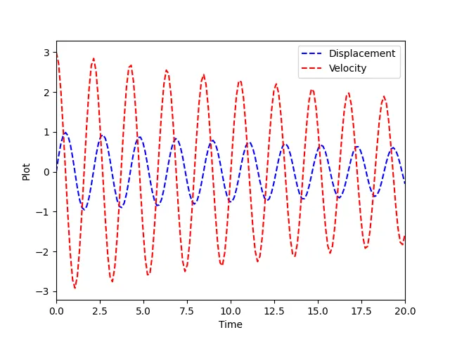
5. Plot Displacement / Velocity vs Time graph.

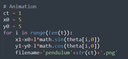
6. Calculate the pendulum position and define file name.

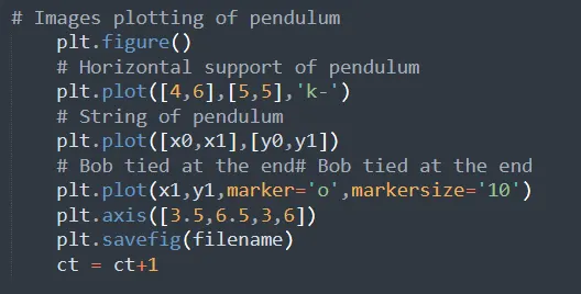
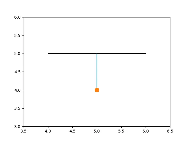
7. Plot the images and save them in different file using string.

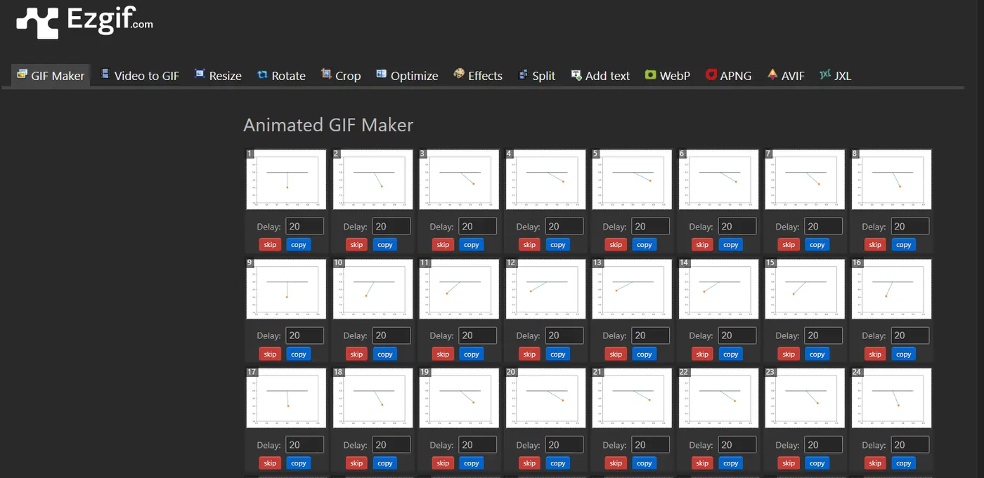
8. Convert the images to animation by going to any online website

Python Code:

# Simulation of motion of Pendulum

# Importing the basic libraries/ modules

import math

import matplotlib.pyplot as plt

import numpy as np

from scipy.integrate import odeint

def model(theta,t,b,g,l,m):

theta1=theta[0]

theta2=theta[1]

dtheta1_dt=theta2

dtheta2_dt=-(b/m)*theta2-(g/l)*math.sin(theta1)

dtheta_dt=[dtheta1_dt,dtheta2_dt]

return dtheta_dt

#Inputs

b = 0.05

g = 9.81

l = 1

m = 1

#Initial Conditions

theta_0 = [0,3]

#Time Points

t = np.linspace(0,20,150)

#Solve the ODE

theta = odeint(model,theta_0,t,args=(b,g,l,m))

# Plotting

plt.plot(t,theta[:,0],'b--',label='Displacement')

plt.plot(t,theta[:,1],'r--',label='Velocity')

plt.xlabel('Time')

plt.ylabel('Plot')

plt.xlim([0,20])

plt.legend(loc='best')

plt.show()

# Animation

ct = 1

x0 = 5

y0 = 5

for i in range(len(t)):

x1=x0+l*math.sin(theta[i,0])

y1=y0-l*math.cos(theta[i,0])

filename='pendulum'+str(ct)+'.png'

# Images plotting of pendulum

plt.figure()

# Horizontal support of pendulum

plt.plot([4,6],[5,5],'k-')

# String of pendulum

plt.plot([x0,x1],[y0,y1])

# Bob tied at the end# Bob tied at the end

plt.plot(x1,y1,marker='o',markersize='10')

plt.axis([3.5,6.5,3,6])

plt.savefig(filename)

ct = ct+1

Result:

Displacement / Velocity vs Time graph

Pendulum Animation

Conclusion: Solving second order ODEs and pendulum motion simulation is done successfully.