Week 3 - Solving second order ODEs
Objective:
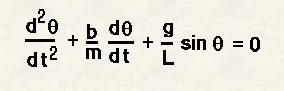
write a program that solves the following ODE
Problem Statement:
ODE is used to describe the transient behavior of a system. The way the pendulum moves depends on the Newtons second law. When this law is written down, we get a second order Ordinary Differential Equation that describes the position of the "ball" w.r.t time.
Solution Procedure:
write a code.
code is explained.
the code is as below:
import numpy as np
from scipy.integrate import odeint
import matplotlib.pyplot as plt
import math
# this is a Python program to simluate pendulum
#factors involved are as follows:
'''
g = gravity in m/s2,
L = length of the pendulum in m,
m = mass of the ball in kg,
b=damping coefficient.
'''
#fucntion that return dTheta/dt - array of displacement and velocity for specfied time interval
def model(theta, t, b, g, l, m):
theta1 = theta[0]
theta2 = theta[1]
dTheta1_dt = theta2
dTheta2_dt = -(b/m) * theta2 - (g/l) * (math.sin(theta1))
dTheta_dt = [dTheta1_dt, dTheta2_dt]
return dTheta_dt
#constants for pendulum
l=1
m=1
b=0.05
g=9.81
#hinje point location
x0 = 0
y0 = 0
#length of string
L = 2
#initial condition definition - angular displacement is 0, initial velocity is 3 rad/sec at time 0 seconds
theta_0 = [0, 3]
#timepoints - 0 to 20 seconds split 150 times
time = np.linspace(0, 20, 150)
#solve ODE - theta is solution having all the values of displacement and velocity
theta = odeint(model, theta_0, time, args = (b, g, l, m))
# theta[:, 0] values ae in degrees
#gpahs to plot the pendulum animation
ct = 1
for value in theta[:, 0]:
xInst = x0 + L * math.sin(value)
yInst = y0 - L * math.cos(value)
fileName = '%05d.png' %(ct)
ct +=1
plt.figure()
plt.plot([x0, xInst], [y0, yInst])
plt.plot(xInst, yInst, 'o', markersize = 20)
plt.xlim([-2, 2])
plt.ylim([-2.5, 0])
plt.savefig(fileName)
plt.close()
#plot reults for displacement and velocity into single graph
plt.plot(time, theta[:, 0], 'b-', label = r'$\frac{d\theta_1}{dt} = \theta2(Displacement)$')
plt.plot(time, theta[:, 1], 'r--', label = r'$\frac{d\theta2}{dt} = -\frac{b}{m}\theta2 - \frac{g}{l}sin\theta1$')
plt.xlabel('time')
plt.ylabel('plot')
plt.legend(loc = 'best')
plt.show()
graphs are plotted. they are explained.
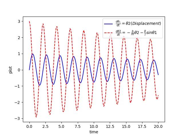
the blue line indicates the angular displacement of the pendulum bob. we can see damping in effect as the displacement decreases over time.
the red dotted line depicts the velocity over time. we can see it decreasing over time as a result of applied damping.
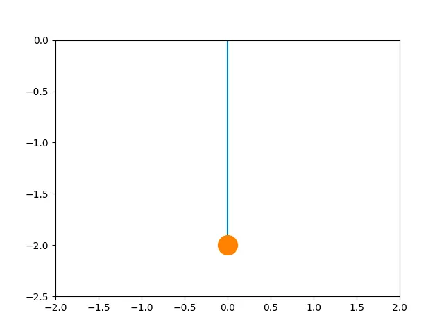
animation of the pendulum in GIF and mp4 is attached herewith.
animation on You tube is published and the You tube link for an animation in your report is provided below:
https://youtu.be/lhBWSDTpUHQ
Results and Discussion:
Objective:
write a program that solves the following ODE
Problem Statement:
ODE is used to describe the transient behavior of a system. The way the pendulum moves depends on the Newtons second law. When this law is written down, we get a second order Ordinary Differential Equation that describes the position of the "ball" w.r.t time.
Solution Procedure:
write a code.
code is explained.
plot graphs. they are explained.
Results and Discussion
Step wise explanation of your code. - this is provided in the code itself.
Errors faced while programming.
plt.plot(time, theta[:, 1], 'r--', label = r'$\frac{d\theta2}{dt} = -\frac{b}{m}\theta2 - \frac{g}{l}sin\theta1$')
error was faced in this line of code.
How have you overcome those errors.
it was solved by properly writing the "\" and "$".
the files are also attached.