Week 3 - Solving second order ODEs

Aim:

To write a Matlab program that will simulate the pendulum motion.

Formula:

Equation of motion of simple pendulum with damping

`(d^2 θ) /( d t )^ 2 + b/ m ( (d θ)/ (d t) ) + ( g/l ) sin θ = 0`

Breaking down second order differential equation to series of first order differential equation:

Second order differential equation of simple pendulum

`(d^2 θ) /( d t )^ 2 + b/ m ( (d θ)/ (d t) ) + ( g/l ) sin θ = 0`

`θ = θ _1`---1

`(d θ)/ (d t) = (d θ_1)/( d t) = θ_2`----2

`(d ^2 θ )/( d t ) ^2 = (d ^2 θ _1)/( d t ^2) = d/ (d t)( ( d θ _1 )/(d t )) = (d )/(d t )( θ _2 )`------3

By substituting (1), (2), (3) in above equation we get

`(d^2 θ_1) /( d t )^ 2 + b/ m ( (d θ_1)/ (d t) ) + ( g/l ) sin θ_1 = 0`

`(d θ_2) /( d t )^ 2 + b/ m ( θ_2 ) + ( g/l ) sin θ_1 = 0`

`(d θ_2) /( d t )^ 2 = -( b/ m ( θ_2 ))-(( g/l ) sin θ_1)`

Coding:

import math
import matplotlib.pyplot as plt
import numpy as np
from scipy.integrate import odeint 

def func_ode(t,t_span,b,g,l,m):
	theta1=t[0]
	theta2=t[1]
	dtheta1_dt=theta2
	dtheta2_dt= (-(b/m)*theta2)-((g/l)*math.sin(theta1))
	Theta=[dtheta1_dt,dtheta2_dt]
	return Theta

#inputs mass-m, gravity-g, length of string-l, damping factor-b.

b=0.05
m=0.1
g=9.81
l=1

theta_0=[0,3]
t_span= np.linspace(0,25,600)
t=odeint(func_ode,theta_0,t_span,args = (b,g,l,m))

#plotting the graph
plt.plot(t_span,t[:,0])
plt.plot(t_span,t[:,1])
plt.legend(["angular displacement","angular velocity"])
plt.xlabel("T-span")
plt.show()

a=t[:,0]
ct=1

for i in a:
	THETA1=i
	x0=0
	y0=0
	x1=l*math.sin(THETA1)
	y1=-l*math.cos(THETA1)

	filename='test%05d.png' % ct
	ct=ct+1

	#plotting the pendulum
	
	plt.figure()
	plt.plot([x0,x1],[y0,y1],linewidth=5)
	plt.plot([-1.5,1.5],[0,0],linewidth=5)
	plt.plot(x1,y1,'o',markersize=20)
	plt.xlim([-1.5,1.5])
	plt.ylim([-1.5,0.25])
	plt.savefig(filename)

Explanation:

From the equation we came to know that, we must initialize the values of mass, gravity, length of string, damping factor as per question. Then the value of angular displacement, and angular velocity initialized as per question. T span is also initialized from 0 to 25 using linspace command to get more values between 0 to 25. Breaking down of second order differential equation to series of first order differential equation is inserted in function. ODEINT solver only solve first order differential equation, so only the second order differential equation is break down to series of first order differential equation. The output is stored in t which contains both angular displacement, and angular velocity value. Next thing is to make the simulation of pendulum using plotting. We need to find the values of x0, x1, y0, y1 using formula and for loop. Here the theta value for plotting is got from values of result. After knowing all values plot it so we get the string of pendulum now we require bob in which its centre should be attached to the end point of string so we need to use other plot command in that we use (o) in which its size can be increased with help of markersize command so that we obtain a bob. To obtain animation we use imagemagick software to stich all the images into a video using command prompt. Then the values of angular displacement and angular velocity is also plotted. Legend command is used to diffrentiate the both curves.

Output:

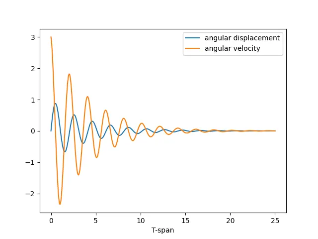
From the above graph, The initial value of angular velocity and angular displacement is 0 and 3 respectively which means pendulum is oscillating,and Due to damping factor it is damped and come to rest position.

Pendulum animation video link:

The animation is done by stiching all the images which we got as output in command prompt using imagemagick

https://drive.google.com/file/d/1CV3UcQPniLEDAmjvSN-fH1WOWJ0Gt2ub/view?usp=sharing

Error faced and overcome:

The error which I faced is the length of the string is changed in different position of pendulum and its is rectified by ranging x-axis and y-axis in plot.