Week 3 - Solving second order ODEs

Objective:

1) To write a program to plot pendulum motion vs time .

2) To write a program to animate motion of pendulum with given properties.

Theory :

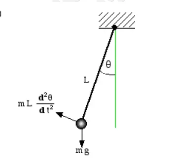
From force balance equation :

`d^2/dt^2 theta` + b/m `d/dt theta` + g/l sin`theta` = 0

Let `theta = theta1`

then , `d/dt theta = d/dt theta1 = theta 2`

`d^2/dt^2 theta = d^2/dt^2 theta1=d/dt(d/dt theta1)=d/dt(theta2)`

`d^2/dt^2 theta + b/m d/dt theta+ g/l sin theta=0`

We can reduce the second order differential equation to 2 first order differential equations

`d/dt theta2 = -b/m theta2 - g/l sin theta1`

where ,

b= damping co-efficient

m=mass

g= acceleration due to gravity

l=length

`theta =`angular displacement

Program logic :

Initially we need to enter values for length , damping co-efficient , acceleration due to gravity and mass

l=1;
b=0.05;
g=9.81;
m=1;

Defining , Initial condition vector at time t=0 . : Given that at time t=0 , angular displacement=0 and angular
theta_0=[0;3] velocity = 3 rad/sec.

To get variable time points from 0 to 20 seconds .
t_span=linspace(0,20,200)

To solve the Ordinary Differentiall Equation , we use ode45 function

[t,results] = ode45(@(t,theta) ode_func(t,theta,b,g,l,m),t_span,theta_0)

We need to define ode_func as :

function[dtheta_dt] = ode_func(t,theta,b,g,l,m)

theta1=theta(1) : to assign theta1 as theta(angular displacement)
theta2=theta(2) : to assign theta 2 as theta (angular velocity)
dtheta1_dt=theta2
dtheta2_dt=-(b/m)*theta2-(g/l)*sin(theta1) : To solve the first order differential equation
dtheta_dt=[dtheta1_dt; dtheta2_dt] : assigning new values to [angular displacement ; angular velocity]

plot(t,results(:,1)) : To plot angular displacement VS Time
hold on : To hold on to plot while creating next plot
plot(t,results(:,2)) : To plot angular velocity VS time

title('Oscillation of a Simple Pendulum') : To Assign title
ylabel('Plot') : To name y axis
xlabel('Time') : To name x axis

displ=results(:,1) : To display all data in first column

Next we need to write code for animation of pendulum motion

ct=1 : To define initial value of counter

for i=1:length(t) : To initiate for loop to change value of i from 0 to 20 sec .

: To define Initial position of pendulum
x0=0;
y0=0;

:To define final position of pendulum

x1=l*sin(displ(i)); : To vary x1 according to value of theta
y1=-l*cos(displ(i)); :To vary y1 according to value of theta in negative Y axis

figure(2)

plot([-1 1],[0 0], 'linewidth',2,'color','r') :To define base line

hold on : To hold on to plot while plotting next plot

line([x0 x1],[y0 y1],'linewidth',2,'color','b') : To plot string of the pendulum

plot(x1,y1, 'marker','o','markersize',25,'MarkerFaceColor','r') : To plot the bob of pendulum according to values of x1,y1

axis([-2 2 -2 2]) : To lock the axes
pause=0.2
title('Motion of a simple Pendulum')
P(ct)=getframe(gcf) : To obtain a frame of the plot for every value of ct
ct=ct+1 : incrementing counter value for next loop

hold off
end : To mark end of for loop

movie(P) : To make movie out of frames created from P
videofile=VideoWriter('Simple_Pendulum.avi','uncompressed AVI') : To define a file for video created in AVI format
open(videofile) : To open videofile
writeVideo(videofile,P) : To write coompile contents of frames from P into a videofile .
close(videofile) : To end the videofile

Codes :

1) Code to plot motion of pendulum and animation of the same

clear all
close all
clc

l=1;
b=0.05;
g=9.81;
m=1;

%Initial condition
theta_0=[0;3];

%time points
t_span=linspace(0,20,200);

%solve ODE 
[t,results] = ode45(@(t,theta) ode_func(t,theta,b,g,l,m),t_span,theta_0);

plot(t,results(:,1))
hold on
plot(t,results(:,2))
title('Oscillation of a Simple Pendulum')
ylabel('Plot')
xlabel('Time')

displ=results(:,1);

%Code for pendulum 
ct=1

for i=1:length(t)
    
    %Initial position of pendulum
    x0=0;
    y0=0;
    
    %Final position of pendulum
    
    x1=l*sin(displ(i));
    y1=-l*cos(displ(i));
    
    figure(2)
    
    %Base line
    plot([-1 1],[0 0], 'linewidth',2,'color','r')
    
    hold on
    %Pendulum string
    line([x0 x1],[y0 y1],'linewidth',2,'color','b')
    
    %Pendulum ball
    plot(x1,y1, 'marker','o','markersize',25,'MarkerFaceColor','r')
    
    %Animation plot
    axis([-2 2 -2 2])
    pause=0.2
    title('Motion of a simple Pendulum')
    P(ct)=getframe(gcf)
    ct=ct+1
    
    hold off
end
%  To create movie file
movie(P)
videofile=VideoWriter('Simple_Pendulum.avi','uncompressed AVI')
open(videofile)
writeVideo(videofile,P)
close(videofile)

2) Codes to define ode_func

function[dtheta_dt] = ode_func(t,theta,b,g,l,m)

theta1=theta(1)
theta2=theta(2)
dtheta1_dt=theta2;
dtheta2_dt=-(b/m)*theta2-(g/l)*sin(theta1);
dtheta_dt=[dtheta1_dt; dtheta2_dt];
end

Results :

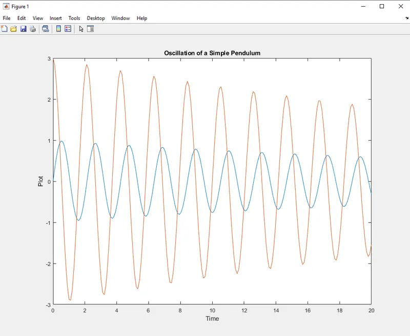
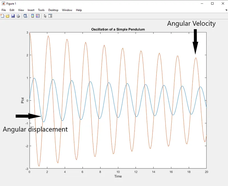
1) The graph showing variation of valocity and displacement with time .

2) The animation for motion of pendulum was created .

Errors Occured :

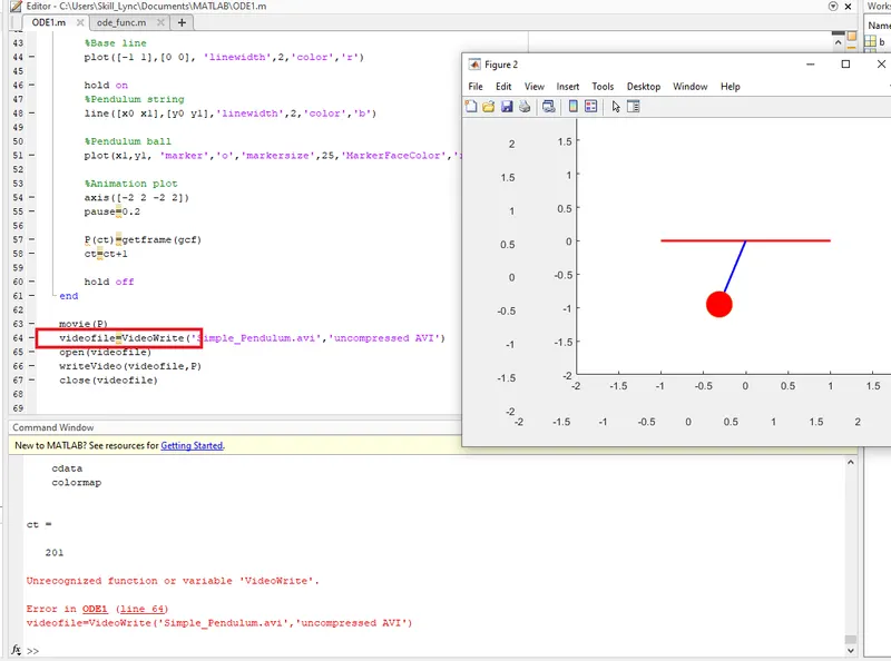
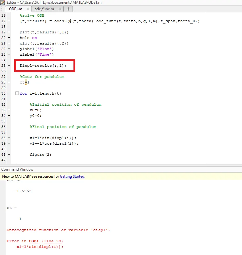
This error occured due to a typo error . Instead of displ , Displ was typed .