Week 3 - Solving second order ODEs

Aim:Solving ordinary differential equation for simulation of simple pendulum.

Objectives:

• To code for motion of simple pendulum and determine the variation of displacement and velocity with respect to time.
• To add animation for realistic data interpretation.
• To vary the inputs of the program and find out a change in outputs.

Introduction:

A pendulum is a body suspended from a fixed support so that it swings freely back and forth under the influence of gravity.

The second order equation for simple pendulum is given by:

d²Ɵ/dt² + (b/m)*dƟ/dt + (g/L)*sin(Ɵ) = 0 -------- (1)

For solving this second order ode in python we can divide it into two first order ode’s:

Ɵ = Ɵ1 -------- (2)

dƟ/dt = dƟ1/dt = Ɵ2 --------- (3)

d²Ɵ/dt² = d/dt*(dƟ/dt)= dƟ2/dt ----------- (4)

Substituting all this equation into equation (1) we get:

dƟ2/dt + (b/m)*Ɵ2 + (g/L)*sin(Ɵ1) = 0

dƟ2/dt = - (b/m)*Ɵ2 – (g/L)*sin(Ɵ1)

so our final equations are:

dƟ1/dt = Ɵ2

dƟ2/dt = - (b/m)*Ɵ2 – (g/L)*sin(Ɵ1)

In matrix format

Ɵ = [ dƟ1/dt , dƟ2/dt ] = [ Ɵ2 , - (b/m)*Ɵ2 – (g/L)*sin(Ɵ1)]

we will use this matrix in our function.

Some of the important parameters to consider while programming for simple pendulum are:

1. Length of wire=1m
2. mass of bob=1kg
3. damping=0.05
4. Acceleration due to gravity=9.81m/s2

Steps to generate a program/logic:

Step1:Insert all the inputs in program

Step2:Define initial condition for displacement and velocity

Step3:Define a time span given in above problem as 10sec

Step4:Using odeint predefined function in python from scipy module,to use odeint we have to pass on a function which should contain formula to calculate the value of theta ,since the simple pendulum equation is second order ode we will get two theta values.

The syntax for odeint in python is:

odeint(func,tspan,y0,arg=())

where,

func = function

tspan=span of time

y0=Initial condition

arg = arguments

Step5:Write a function to calculate values of theta.

Step6:plot displacement and velocity with respect to time.

Step7:Create a for loop to generate different position of pendulum by iterating it with different values of 'i'

Step8:Pass on the values of (XO,YO) and formula to calculate value of (X1,Y1)

Step9:plot for (XO,YO) which is fixed point and (X1,Y1) with varying values.

Step10:To create animation we can use image magick.

Python code for simulation of simple pendulum:

import numpy as np
import math
import matplotlib.pyplot as plt 
from scipy.integrate import odeint


#code to solve simple pendulum ode
#function to calculate theta
def simple_pendulum(theta,t,b,g,m,L):
	
	dtheta_dt = [theta[1], (-(b/m)*theta[1] -(g/L)*math.sin(theta[0]))]
	return dtheta_dt

#inputs
b = 0.02 #damping
g = 9.81 # acceleration due to gravity
m = 0.1 #mass in kg
L = 1 #length of string in meters

 #initial condition
theta_0  = [math.pi/2,0]

 #time array
t = np.linspace(0,10,150)	

theta = odeint(simple_pendulum,theta_0,t,args = (b,g,m,L))

#plotting displacement and velocity with respect to time
plt.plot(t,theta[:,0],'--r',label= r'$\frac{d\theta1}{dt} = \theta_2$')
plt.plot(t,theta[:,1],'o-b',ms = 3,label= r'$\frac{d\theta2}{dt} = -\frac{b}{m}\theta_2 - \frac{g}{L}\sin(\theta_1)$')
plt.legend(loc='best')
plt.ylabel('disp and vel')
plt.xlabel('time')
plt.title('variation of velocity and displacement of simple pendulum')
plt.savefig('SHM.png')

#calculating the array of theta value for animation
theta_anim = theta[:,0]
ct =1
#loop to calculate (x1,y1) at different theta values
for theta in theta_anim:
	theta_new = theta
	x0 = 0
	y0 = 2.5
	x1 = L*math.sin(theta_new)
	y1 = -(L*math.cos(theta_new))
	filename = 'simple_pend%03d.png' % ct
	ct = ct + 1

#Plotting for animation
	plt.figure()
	plt.plot([x0,x1],[y0,y1],lw = 2)
	plt.plot(x1,y1,'o-r',ms = 30)
	plt.plot([-1,-0.5],[2.5,2.5],'-k',lw = 5)
	plt.plot([-0.5,0.5],[2.5,2.5],'-k',lw = 5)
	plt.plot([0.5,1],[2.5,2.5],'-k',lw = 5)
	plt.plot([-1,-0.5],[3,3],'-k',lw = 5)
	plt.plot([-0.5,0.5],[3,3],'-k',lw = 5)
	plt.plot([0.5,1],[3,3],'-k',lw = 5)
	plt.plot([-0.5,-0.5],[2.5,3],'-k',lw = 5)
	plt.plot([0.5,0.5],[2.5,3],'-k',lw = 5)
	plt.xlim([-3,3])
	plt.ylim([-2,4])		
	plt.savefig(filename)

Plot:

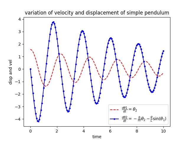
This plot explains the variation of displacement and velocity with respect to time and how it goes on decreases with time which is directly proportional to damping co-efficient.

Animation of simple pendulum:

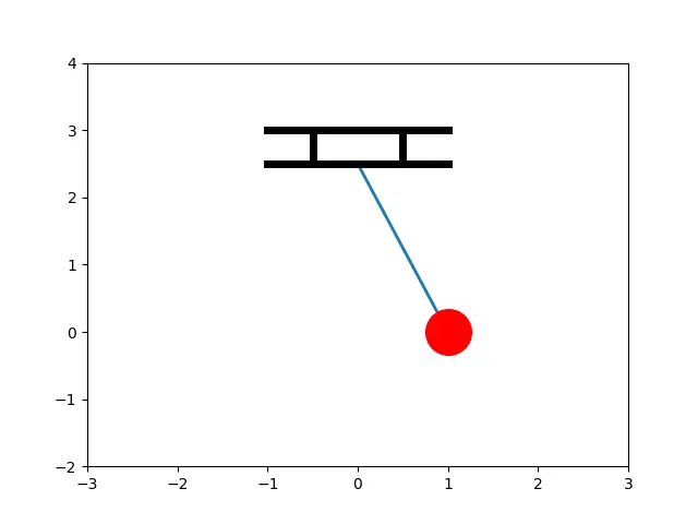
link for animation:

https://drive.google.com/file/d/17J34Ota030dmHo1DUZCSD3aVhA4jPLrF/view?usp=sharing

Conclusion:

As the damping co-efficient increases the displacement and velocity decreases rapidly.

This is the case of over damping.

If we can solve second order ode then we can able to solve many processes one of which is the spring, damper and mass system. for which same equation holds good we can find out the correct amount of damping and spring stiffness which should be used in automobiles.