To write a MATLAB program to simulate a simple Pendulum by using the second-order ordinary differential equation (ODE).

AIM OF THE PROJECT:

To write a MATLAB program to simulate a simple Pendulum by using the second-order ordinary differential equation (ODE).

INTRODUCTION:

In simple word, an arrangement of the suspended mass with the help of a string which is attached with a wall (here, the mass of the string is generally considered as zero) is defined by the simple pendulum. Usually, the position of the suspended mass of the pendulum is shown by the below written second-order ordinary differential equation or ODE.

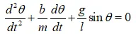
In Engineering, ODE is used to describe the transient behavior of a system. A simple example is a pendulum. The way the pendulum moves depends on Newton's second law. When this law is written down, we get a second order Ordinary Differential Equation that describes the position of the "ball" w.r.t time.

OBJECTIVE OF THE PROJECT:

The main objective of this project is to write a MATLAB code to simulate a simple Pendulum by using the second-order ordinary differential equation (ODE).

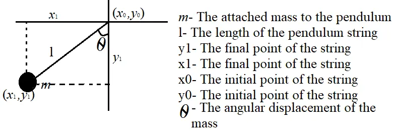
REQUIRED DIAGRAM:

GOVERNING EQUATIONS:

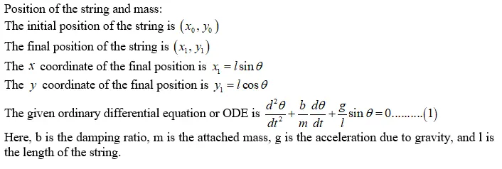
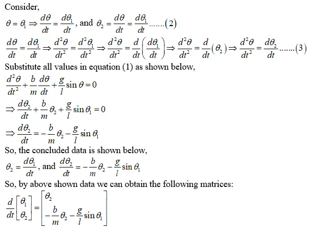
Damping Ratio (b)- In simple word, the damping ratio is a kind of dimensionless quantity which describes the process of the decay of the oscillation of a system after some disturbance. In engineering, we can find either an underdamped system, an overdamped system, or a critically damped system.

ASSUMPTION OF THE INPUT DATA:

The length of the pendulum is l = 1 m

The mass of the attached mass is m = 1 kg

The damping ratio is b = 0.05

The acceleration due to gravity is g = 9.81 meter per second square

The given time span is 0 to 20 seconds

The angular velocity is 0 to 3 radian per second

The angular displacement is 0 to 3

MATLAB PROGRAM:

ODE45 command- This command is generally used to solve an ordinary differential equation or ODE.

Simple MATLAB program to solve the differential equation and plot the simple graph is:

clear all

close all

clc

%Input data

%Length (m) of the pendulum is:

l = 1;

%Mass (kg) of the ball is:

m = 1;

%Damping coefficient is:

b = 0.05

%Acceleration due to gravity (m/s^2) is:

g = 9.81;

%Angular vellocity (rad/sec) is:

theta_0 = [0;3];

%time span (second) is:

t_span = linspace(0,20,500);

%Relation needed to solve ordinary differential equation is:

[t,results] = ode45(@(t,theta) ode_func(t,theta,b,g,l,m),t_span,theta_0);

hold on

%Plotting of graph is:

figure(1)

plot(t,results(:,1));

plot(t,results(:,2));

ylabel('plot')

xlabel('time')

grid on

hold off

The MATLAB program of the used function is:

function[dtheta_dt] = ode_func(t,theta,b,g,l,m)

theta1 = theta(1);

theta2 = theta(2);

dtheta1_dt = theta2 ;

dtheta2_dt = (-b/m)*theta2-(g/l)*sin(theta1);

dtheta_dt = [ dtheta1_dt;dtheta2_dt];

end

Simple OUTPUT of the program is:

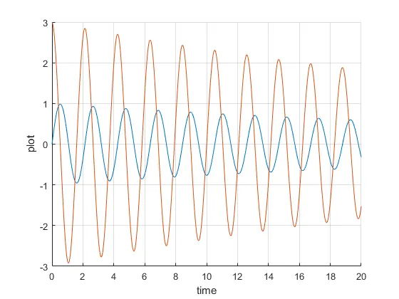
MATLAB program to simulate a simple Pendulum by using the second-order ordinary differential equation (ODE)

clear all

close all

clc

%Input data

%Length (m) of the pendulum is:

l = 1;

%Mass (kg) of the ball is:

m = 1;

%Damping coefficient is:

b = 0.05

%Acceleration due to gravity (m/s^2) is:

g = 9.81;

%Angular vellocity (rad/sec) is:

theta_0 = [0;3];

%time span (second) is:

t_span = linspace(0,20,500);

%Relation needed to solve ordinary differential equation is:

[t,results] = ode45(@(t,theta) ode_func(t,theta,b,g,l,m),t_span,theta_0);

hold on

%Plotting of graph is:

figure(1)

plot(t,results(:,1));

plot(t,results(:,2));

ylabel('plot')

xlabel('time')

grid on

hold off

ct = 1;

%Plot data for creating animation of the pendulum:

for i = 1:length(results(:,1))

    THETA = results(i,1);

    %Initial point of pendulum:

    x0 = 0;

    y0 = 0 ;

    %Final point of pendulum:

    x1 = 1*sin(THETA);

    y1 = -1*cos(THETA);

    %Plot the pendulum:

    figure(2)

    %First of all plot the wall in which the string of the pendulum will be

    %attached:

    plot ([-1 1],[0 0],'linewidth',5);

    hold on

    %Now, plot the string of the pendulum:

    plot ([ x0,x1],[y0,y1],'linewidth',3,'color','r');

    hold on

    %Now, plot and attached the mass with O marker:

    plot (x1,y1,'O','markersize',25,'markerFacecolor','black')

    axis([-1.5 1.5 -1.5 1 ])

    pause(0.02)

    grid on

    hold off

      M(ct) = getframe(gcf);

      ct= ct+1;

end

%Obtain the animation by using the following command:

movie(M)

  videofile = VideoWriter('pendulum_Animation.avi','uncompressed avi');

  open (videofile)

  writeVideo(videofile,M)

   close (videofile)

In this program, we can use the function written in the sample program.

OUTPUT:

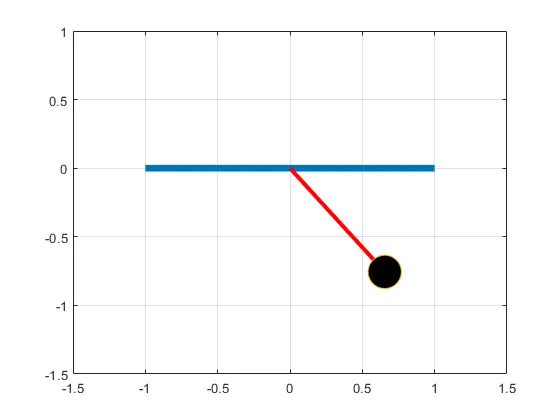
Animation link:- https://youtu.be/vz-1L7gaTlE

CONCLUSION:

The curve between the angular displacement and the angular velocity is plotted.

REFERENCES:

1. http://hyperphysics.phy-astr.gsu.edu/hbase/pend.html#:~:text=A%20simple%20pendulum%20is%20one,For%20pendulum%20length
2. https://www.math24.net/nonlinear-pendulum/
3. https://math.libretexts.org/Bookshelves/Calculus/Book%3A_Calculus_(OpenStax)/17%3A_Second-Order_Differential_Equations/17.3%3A_Applications_of_Second-Order_Differential_Equations