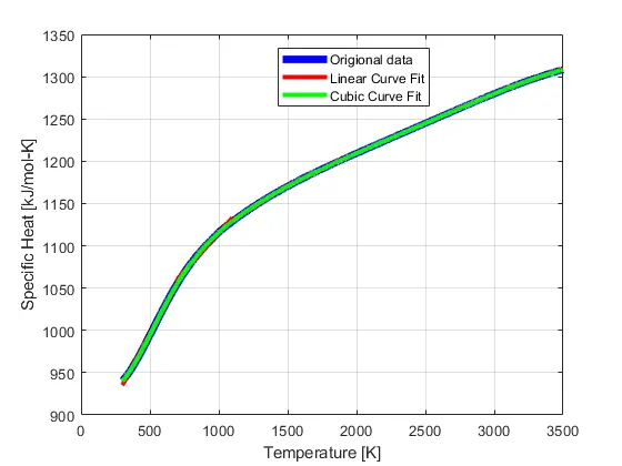
A MATLAB program to fit a linear and cubic polynomial for the specific heat or Cp data.

Aim of the Project:

To write a MATLAB program to fit a linear and cubic polynomial for the specific heat or Cp data.

Introduction:

Curve Fitting- In simple words, curve fitting is a process of constructing a mathematical function or a curve that posses the nearest proximity to the given real series of various data. By using the curve fitting method, we can mathematically construct the mathematical relationship between the parameter values and the observed dataset. For the modeling of some natural processes, curve fitting is a highly effective mathematical method.

Objective of the Project:

The main objective of this project is to write a MATLAB program to fit a linear and cubic polynomial for the specific heat or Cp data and plot the linear and cubic fit curves along with the raw data points.

Required Diagram:

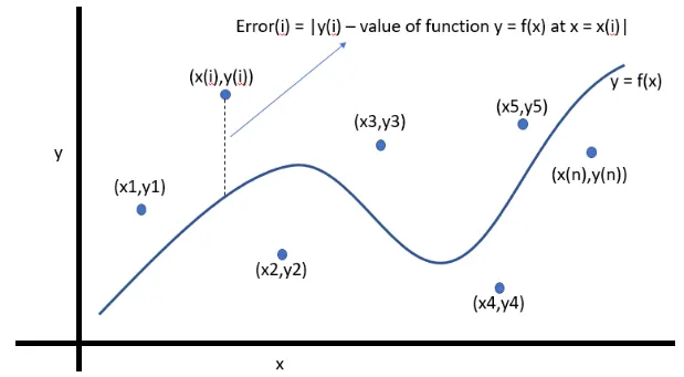
Figure- (1)

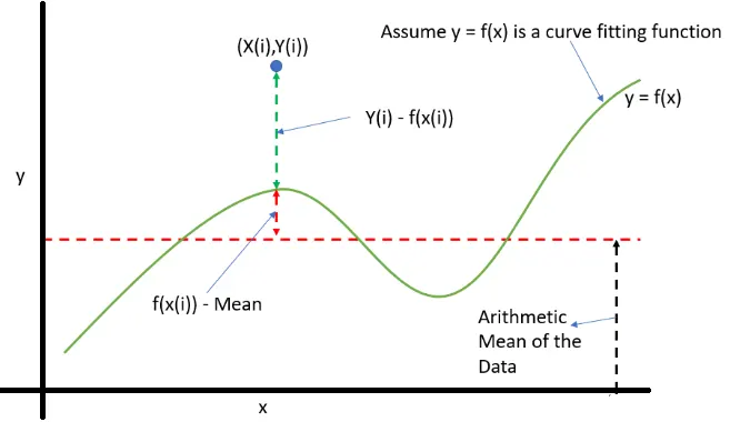
Figure-(2)

Governing Equations:

How to choose a curve is the best fit for the given set of data- Generally, we are using below shows four steps to finding a curve that satisfies the data points.

1. SSE (Sum of square due to errors)
2. R square
3. Adjusted value of the R square
4. RMSE (Root mean square error)

R Square- In simple words, the R square is a quantity that measures how successful the given fit is explaining the changing or variation of the data if it seems the higher value of R square is a better fit and the lower value is the bad fit for the set of data. The numerical value of the R square varies between zero (0) and one (1). Usually, the following relation is used to determine the R square value.

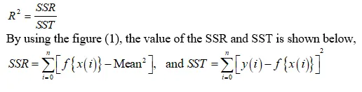
Sum of square due to errors (SSE):

The Sum of square due to errors is the sum of the SST and SSR

Root mean square error (RMSE):

The mathematical expression needed to calculate the Root mean square error is shown below,

In the above-shown formula, n stands for the total number of data points.

MATLAB Program:

Simple MATLAB program to plot the given set of the specific heat data with the linear set:

clear all

 close all

 clc

  %preparing data

 Cp_data = load('data');

 Temperature = Cp_data(:,1);

 Specific_Heat = Cp_data(:,2);

 %plot the data

 plot(Temperature, Specific_Heat, 'linewidth',3,'color','b')

 xlabel('Temperature [K]')

 ylabel('Specific Heat [kJ/mol-K]')

 %Curve fitting

 %Specific_Heat = a*T^2 + b*T +

 co_effs = polyfit(Temperature,Specific_Heat,1);

 predicted_specific_heat = polyval(co_effs,Temperature);

 hold on

 plot(Temperature, predicted_specific_heat, 'linewidth',3,'color','r')

 legend('Origional data set','Curve fitted data')

 grid on

OUTPUT:

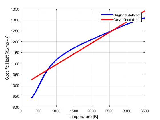
Simple MATLAB program to plot the given set of the specific heat data with the cubic set:

clear all

 close all

 clc

  %preparing data

 Cp_data = load('data');

 Temperature = Cp_data(:,1);

 Specific_Heat = Cp_data(:,2);

 %plot the data

 plot(Temperature, Specific_Heat, 'linewidth',3,'color','b')

 xlabel('Temperature [K]')

 ylabel('Specific Heat [kJ/mol-K]')

 %Curve fitting

 %Specific_Heat = a*T^2 + b*T +

 co_effs = polyfit(Temperature,Specific_Heat,2);

 predicted_specific_heat = polyval(co_effs,Temperature);

 hold on

 plot(Temperature, predicted_specific_heat, 'linewidth',3,'color','r')

 legend('Origional data set','Curve fitted data')

 grid on

OUTPUT:

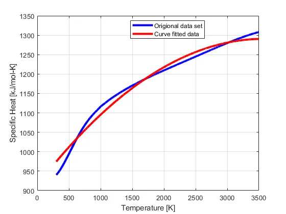
MATLAB program for both cubic and linear polynomial without splitting the data.

clear all

close all

clc

%preparing data

 Cp_data = load('data');

 Temperature = Cp_data(:,1);

 Specific_Heat = Cp_data(:,2);

 x = mean(Specific_Heat);

 n = 8;

  %Linear Curve fitting

 %Specific_Heat = a*T^2 + b*T +

 co_effs1 = polyfit(Temperature,Specific_Heat,1);

 predicted_specific_heat1 = polyval(co_effs1,Temperature);

 %Split the data points

 a = 1;

 b = 3200/n;

 for i = 1:n

   co_effs1_split = polyfit(Temperature(a:b),Specific_Heat(a:b),1);

   predicted_specific_heat1_split(a:b) = polyval(co_effs1_split,Temperature(a:b));

   a = b + 1;

   b = b + (3200/n);

 end

 %plot the data points

 plot(Temperature, Specific_Heat, 'linewidth',5,'color','b')

 hold on

 plot(Temperature,predicted_specific_heat1_split,'linewidth',3,'color','r')

 grid on

 %Calculate the value of the R square for linear fit for the split

 %Consider SSR1 = 0, and SSE1 = 0

 SSR1 = 0;

 SSE1 = 0;

 for j = 1:length(Specific_Heat)/n

     SSR1 = SSR1 + (predicted_specific_heat1_split(j)-x).^2;

     SSE1 = SSE1 + (Specific_Heat(j) - predicted_specific_heat1_split(j)).^2;

     R_square1 = SSR1/(SSR1+SSE1);

     RMSE1 = (SSE1/length(Specific_Heat)).^0.5;

 end

 xlabel('Temperature [K]')

 ylabel('Specific Heat [kJ/mol-K]')

 %Cubic Curve fitting

 %Specific_Heat = a*T^2 + b*T +

 co_effs2 = polyfit(Temperature,Specific_Heat,3);

 predicted_specific_heat2 = polyval(co_effs2,Temperature);

 %Split the data points again

 a = 1;

 b = 3200/n;

 for i = 1:n;

     co_effs2_split = polyfit(Temperature(a:b),Specific_Heat(a:b),3);

     predicted_specific_heat2_split(a:b) = polyval(co_effs2_split,Temperature(a:b));

     a = b + 1;

     b = b + (3200/n);

 end

  plot(Temperature,predicted_specific_heat2_split,'linewidth',3,'color','g')

 %Calculate the value of the R square for linear fit for the split

 %Consider SSR1 = 0, and SSE1 = 0

 SSR2 = 0;

 SSE2 = 0;

 for j = 1:length(Specific_Heat)/n

     SSR2 = SSR2 + (predicted_specific_heat2_split(j)-x).^2;

     SSE2 = SSE2 + (Specific_Heat(j) - predicted_specific_heat2_split(j)).^2;

     R_square2 = SSR2/(SSR2+SSE2);

     RMSE2 = (SSE2/length(Specific_Heat)).^0.5;

 end

 xlabel('Temperature [K]')

 ylabel('Specific Heat [kJ/mol-K]')

 legend('Origional data','Linear Curve Fit','Cubic Curve Fit')

OUTPUT: