A MATLAB program to generate the PV diagram of the OTTO Cycle used for the petrol or gasoline engine

AIM OF THE PROJECT:

To write a MATLAB program to generate the PV diagram of the OTTO Cycle used for the petrol engine.

INTRODUCTION:

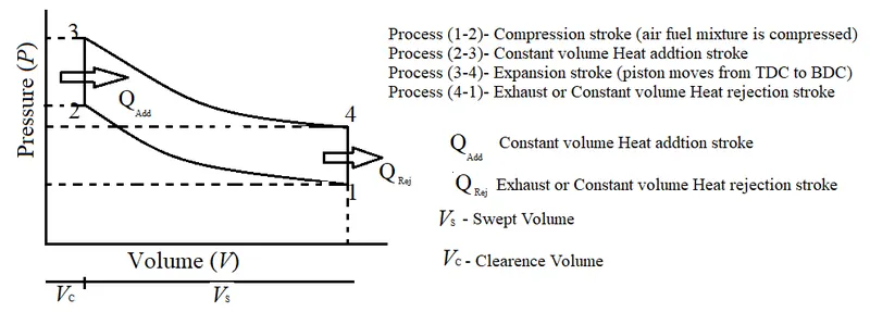
In simple words, the Otto cycle is a simple type of ideal thermodynamic cycle that is generally used to determine the efficiency of a heat engine (mainly for petrol and gasoline engine). This cycle also describes the variation in the mass of the fluid due to the variation in the pressure, temperature, and volume of the fuel. The pressure, temperature, and volume of the fuel varies due to either the addition of the heat or rejection of the heat. In an Otto cycle mainly four processes occur or this cycle has four stages. These stages are shown below,

1. Process 1 to 2- Compression (Isentropic compression)- In this process, the mixture of the fuel (petrol or gasoline) and the air are compressed due to the first stroke or movement of the piston from the bottom dead center to the top dead center of the engine. During this process, the volume of the charge (a mixture of air and fuel) decreases, and its temperature increases.
2. Process 2 to 3- Combustion (Constant volume heat addition)- In this process, the compressed charge is ignited due to the spark plug, and the piston of the engine stays in the top dead center of the engine. This stroke of the engine is also known as a power stroke. In this process the volume of the charge is constant.
3. Process 3 to 4- Expansion (Isentropic expansion)- In this process, the piston of the engine moves from the top dead center to the bottom dead center. During this process, the heat expansion from the engine occurs. During this process, the volume of the charge (a mixture of air and fuel) increases, and its temperature decreases.
4. Process 4 to 1- Exhaust (Constant volume heat rejection- In this process, the heat is released from the engine to the surrounding.

OBJECTIVE OF THE PROJECT:

In this project mainly we have to generate the pressure-volume or PV diagram of the Otto cycle and try to check how the pressure and volume of the charge change. For this, we will use MATLAB software and create a MATLAB program.

REQUIRED DIAGRAM:

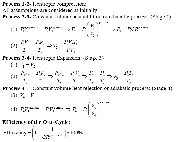
GOVERNING EQUATION:

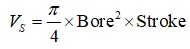
Swept Volume- In simple words, the total volume covered by the piston during its movement from the bottom dead center to the top dead center or vice versa is known as swept volume. The mathematical formula needed to determine the swept volume of an engine is shown below,

Clearance Volume- The total volume between the head of the cylinder and piston when the piston stays in the top dead center is known as clearance volume. The mathematical formula needed to determine the clearance volume of an engine is shown below,

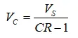
Compression Ratio- The ratio of the total volume of the fuel at the initial point and the total volume of the fuel after compression is generally known as the compression ratio. The mathematical formula needed to determine the compression ratio is shown below,

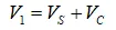
Initial Volume- The summation or total of the swept volume and clearance volume of an engine. Its mathematical form is shown below,

Final Volume- The clearance volume of the engine is the final volume after compression. Its mathematical form is shown below,

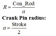
Value of the ratio:

It is the ratio of the connecting rod length and crankpin radius.

ASSUMPTION OF THE INPUT DATA:

gamma = 1.4

T3 = 2300

P1 = 101325

T1 = 500

Bore = 0.1

Stroke = 0.1

Con_Rod = 0.15

CR = 12

MATLAB PROGRAM:

The program needed to plot the point:

clear all

close all

clc

%Input Data of the Engine:

gamma = 1.4;

T3 = 2300;

%State Variable at Point 1:

P1 = 101325;

T1 = 500;

%Geometric Parameters of the Engine:

Bore = 0.1;

Stroke = 0.1;

Con_Rod = 0.15;

CR = 12;

%Calculate Swept and Clearence Volume:

V_Swept = (pi/4)*Bore^2*Stroke;

V_Clearence = V_Swept/(CR-1);

V1 = V_Swept + V_Clearence;

V2 = V_Clearence;

%State Variable at Point 2:

%P2V2^gamma = P1V1^gamma | P2 = P1(V1/V2)^gamma | P2 = P1*CR^gamma

P2 = P1*CR^gamma;

%P1V1/T1 = P2V2/T2 | T2 = P2*V2*T1/(P1*V1)

T2 = P2*V2*T1/(P1*V1);

%State Variable at Point 3:

V3 = V2;

%P3V3/T3 = P2V2/T2 | P3V3/T3 = P2V3/T2 | P3 = P2V3T3/T2V3 | P3 = P2*T3/T2

P3 = P2*T3/T2;

%State Variable at Point 4:

V4 = V1;

%P4V4^gamma = P3V3^gamma | P4 = P3(V3/V4)^gamma

P4 = P3*(V3/V4)^gamma;

%P-V diagram of the Otto cycle

figure(1)

hold on

plot(V1,P1,'*','color','r')

plot(V2,P2,'*','color','r')

plot(V3,P3,'*','color','r')

plot(V4,P4,'*','color','r')

ylabel('Pressure-P')

xlabel('Volume-V')

figure (2)

plot([V1 V2 V3 V4 V1],[P1 P2 P3 P4 P1],'color','b')

ylabel('Pressure-P')

xlabel('Volume-V')

%Thermal efficiency of the Otto Cycle

Efficiency = (1 - (1/CR^(gamma-1)))*100

OUTPUT:

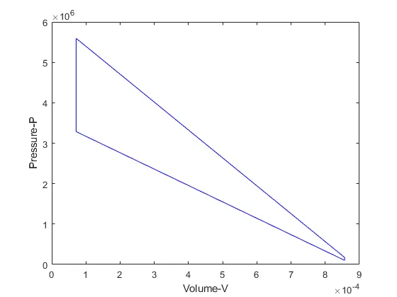
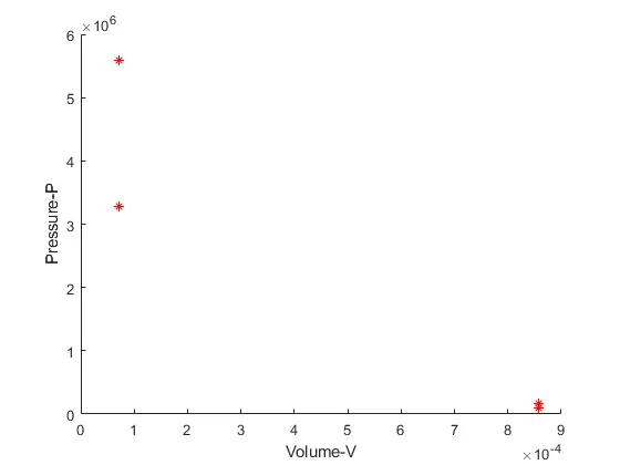
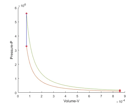
If we will run the above-shown program then we will get the wrong graph or diagram. So, we have to use the following function and include it in the main program to obtain the correct diagram. For the crating function program, we have to use the engine kinematic formula as shown in the governing equation data.

MATLAB program for needed function:

function[V] = OTTOCYCLE_KINEMATICS(Bore, Stroke, Con_Rod, CR, Start_Crank, End_Crank)

a = Stroke/2;

R = Con_Rod/a;

%Calculate Swept and Clearence Volume:

V_Swept = (pi/4)*Bore^2*Stroke;

V_Clearence = V_Swept/(CR-1);

%Angletheta

theta = linspace(Start_Crank, End_Crank, 100);

term1 = 0.5*(CR-1);

term2 = R + 1 -cosd(theta);

term3 = (R^2 - sind(theta).^2).^0.5;

V = V_Clearence*(1 + term1*(term2 - term3))

end

Main MATLAB program to obtain the correct plot:

clear all

close all

clc

%Input Data of the Engine:

gamma = 1.4;

T3 = 2300;

%State Variable at Point 1:

P1 = 101325;

T1 = 500;

%Geometric Parameters of the Engine:

Bore = 0.1;

Stroke = 0.1;

Con_Rod = 0.15;

CR = 12;

%Calculate Swept and Clearence Volume:

V_Swept = (pi/4)*Bore^2*Stroke;

V_Clearence = V_Swept/(CR-1);

V1 = V_Swept + V_Clearence;

V2 = V_Clearence;

%State Variable at Point 2:

%P2V2^gamma = P1V1^gamma | P2 = P1(V1/V2)^gamma | P2 = P1*CR^gamma

P2 = P1*CR^gamma;

%P1V1/T1 = P2V2/T2 | T2 = P2*V2*T1/(P1*V1)

T2 = P2*V2*T1/(P1*V1);

%Use function for compression as shown below

Constant_C = P1*V1^gamma;

V_Compression = OTTOCYCLE_KINEMATICS(Bore, Stroke, Con_Rod, CR, 180, 0);

P_Compression = Constant_C./V_Compression.^gamma;

%State Variable at Point 3:

V3 = V2;

%P3V3/T3 = P2V2/T2 | P3V3/T3 = P2V3/T2 | P3 = P2V3T3/T2V3 | P3 = P2*T3/T2

P3 = P2*T3/T2;

%Use function for expansion as shown below

Constant_C = P3*V3^gamma;

V_Expansion = OTTOCYCLE_KINEMATICS(Bore, Stroke, Con_Rod, CR, 0, 180);

P_Expansion = Constant_C./V_Expansion.^gamma;

%State Variable at Point 4:

V4 = V1;

%P4V4^gamma = P3V3^gamma | P4 = P3(V3/V4)^gamma

P4 = P3*(V3/V4)^gamma;

%P-V diagram of the Otto cycle

figure(1)

hold on

plot(V1,P1,'*','color','r')

plot(V_Compression, P_Compression)

plot(V2,P2,'*','color','r')

plot(V3,P3,'*','color','r')

plot(V_Expansion, P_Expansion)

plot(V4,P4,'*','color','r')

plot([V2 V3],[P2 P3],'color','b')

plot([V4 V1],[P4 P1],'color','b')

ylabel('Pressure-P')

xlabel('Volume-V')

figure (2)

plot([V1 V2 V3 V4 V1],[P1 P2 P3 P4 P1],'color','b')

ylabel('Pressure-P')

xlabel('Volume-V')

%Thermal efficiency of the Otto Cycle

Efficiency = (1 - (1/CR^(gamma-1)))*100

OUTPUT:

CONCLUSION:

The total efficiency of the Otto cycle is 62.9893 percentage

The total area bounded by the curve indicates the total work done

The plotted curve may be used to determine the performance of the engine

References:

• https://www.slideshare.net/mechanical86/dja3032-chapter-2
• https://www.slideshare.net/hm61213/chapter-5-internalcombustionengine
• https://www.princeton.edu/~humcomp/sophlab/ther_28.htm#:~:text=(b)%20The%20%22Clearance%20volume,compression%20ratio%20of%20the%20engine.