Challenge

A MATLAB program to optimize the stalagmite function (Using Genetic Algorithm) and determine the global maxima of that function.

MMd Osama6 Dec 2020

AIM: To write a MATLAB program to optimize the stalagmite function and determine the global maxima of that function.

INTRODUCTION:

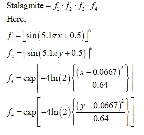
Stalagmite Mathematical Model- It is a mathematical model utilized to improve the local Minima or Maxima. Here for determining the best solution of the Minima or Maxima of the function, we need to utilize the Genetic Algorithm method. In other words, Stalagmite structures are produced from the cave floor that looks upward. Stalagmite functions are mathematical functions that describe the shapes similar to that of the stalagmite and stalactite functions. The mathematical expressions of the stalagmite functions are shown below,

Genetic Algorithm- Generally, this algorithm works on Darwin’s theory of evolution. The genetic algorithm is a technique for solving constrained and unconstrained optimization difficulties based on genetic or natural selection, driving biological development or evolution. The genetic algorithm regularly transforms or modifies a population of particular solutions. At every level, the genetic algorithm chooses individuals at random from the current population to be parents and utilizes them to create children's next generation. Over succeeding generations, the population "grows" near an optimal solution. You can utilize the genetic algorithm to determine several optimization difficulties that are not entirely suited for conventional optimization algorithms, including difficulties in which the objective function is non-differentiable or highly nonlinear. The genetic algorithm can mark difficulties of mixed-integer programming, where some elements are restricted to be integer-valued.

The genetic algorithm utilizes three main kinds of laws at every step to produce the next generation from the current generation or population:

Selection rules- It picks the individuals, called parents, that provide to the next generation's population.
Crossover rules- It connects two parents to create children for the next generation.
Mutation rules- It applies random adjustments to individual parents to create children.

Optimization- Optimization is a Domain of research utilized to Minimize or Maximize a particular function, which depends on various parameters to obtain the desired output.

Syntax of Genetic algorithm (GA):

x = ga(fun,nvars)
x = ga(fun,nvars,A,b)
x = ga(fun,nvars,A,b,Aeq,beq)
x = ga(fun,nvars,A,b,Aeq,beq,lb,ub)
x = ga(fun,nvars,A,b,Aeq,beq,lb,ub,nonlcon)
x = ga(fun,nvars,A,b,Aeq,beq,lb,ub,nonlcon,options)
x = ga(fun,nvars,A,b,[ ],[ ],lb,ub,nonlcon,IntCon)
x = ga(fun,nvars,A,b,[ ],[ ],lb,ub,nonlcon,IntCon,options)
x = ga(problem)
[x,fval] = ga(___)
[x,fval,exitflag,output] = ga(___)
[x,fval,exitflag,output,population,scores] = ga(___)

Explanation of the Syntax:

x = ga(fun,nvars) finds a local unconstrained minimum, x, to the objective function, fun. nvars is the dimension (number of design variables) of fun.

x = ga(fun,nvars,A,b) finds a local minimum x to fun, subject to the linear inequalities A*x ≤ b. ga evaluates the matrix product A*x as if x is transposed (A*x').

x = ga(fun,nvars,A,b,Aeq,beq) finds a local minimum x to fun, subject to the linear equalities Aeq*x = beq and A*x ≤ b. (Set A=[] and b=[] if no linear inequalities exist.) ga evaluates the matrix product Aeq*x as if x is transposed (Aeq*x').

x = ga(fun,nvars,A,b,Aeq,beq,lb,ub) defines a set of lower and upper bounds on the design variables, x, so that a solution is found in the range lb ≤ x ≤ ub. (Set Aeq=[] and beq=[] if no linear equalities exist.)

x = ga(fun,nvars,A,b,Aeq,beq,lb,ub,nonlcon) subjects the minimization to the constraints defined in nonlcon. The function nonlcon accepts x and returns vectors C and Ceq, representing the nonlinear inequalities and equalities respectively. ga minimizes the fun such that C(x) ≤ 0 and Ceq(x) = 0. (Set lb=[] and ub=[] if no bounds exist.)

x = ga(fun,nvars,A,b,Aeq,beq,lb,ub,nonlcon,options) minimizes with the default optimization parameters replaced by values in options. (Set nonlcon=[] if no nonlinear constraints exist.) Create options using optimoptions.

x = ga(fun,nvars,A,b,[],[],lb,ub,nonlcon,IntCon) or x = ga(fun,nvars,A,b,[],[],lb,ub,nonlcon,IntCon,options) requires that the variables listed in IntCon take integer values.

x = ga(problem) finds the minimum for problem, a structure described in problem.

[x,fval] = ga(___), for any previous input arguments, also returns fval, the value of the fitness function at x.

[x,fval,exitflag,output] = ga(___) also returns exitflag, an integer identifying the reason the algorithm terminated, and output, a structure that contains output from each generation and other information about the performance of the algorithm.

[x,fval,exitflag,output,population,scores] = ga(___) also returns a matrix population, whose rows are the final population, and a vector scores, the scores of the final population.

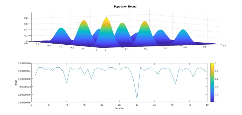
OBJECTIVE: In this project, we need to write a proper MATLAB program to optimize the stalagmite function and determine the global maxima of that function, and plot of all three studies and for F maximum vs the number of iterations.

STOPPING CRITERIA OF THE PROGRAM:

Generations- The algorithm terminates when the number of generations equals the value of Generations.
Time limit- The algorithm terminates after running for an amount of time (in seconds), similar to the time limit.
Fitness limit- The algorithm terminates when the fitness function's value for the current population's best point is smaller than or equal to the Fitness limit.

MATLAB PROGRAM:

MATLAB program for generating the Stalagmite function:

%Stalagmite Function.

function [f]= stalagmite_func(Input_Vector)

x=Input_Vector(1);

y=Input_Vector(2);

f1= (sin(5.1*pi*x+0.5))^6;

f2=(sin(5.1*pi*y+0.5))^6;

f3=exp((-4*log(2))*((x-0.0667)^2/0.64));

f4=exp((-4*log(2))*((y-0.0667)^2/0.64));

f =-(f1.*f2.*f3.*f4);

end

MATLAB program for optimization of a random value and checking the stalagmite function:

%Start the MATLAB program

clear all

close all

clc

%First of all we need to create one dimensional array

x = linspace(0,0.6,150);

y = linspace(0,0.6,150);

%Now create two dimensional array using meshgrid command

[xx, yy] = meshgrid(x,y);

%Now, evaluate the stalagmite function for this we have to use nested for

%loop

for i = 1:length(xx)

    for j = 1:length(yy)

        Input_Vector(1) = xx(i,j);

        Input_Vector(2) = yy(i,j);

        f(i,j) = -stalagmite_func(Input_Vector);

    end

end

surf(xx,yy,f)

shading interp

xlabel('x-value')

ylabel('y-value')

colorbar()

[x_output, fval] = ga(@stalagmite_func,2);

OUTPUT:

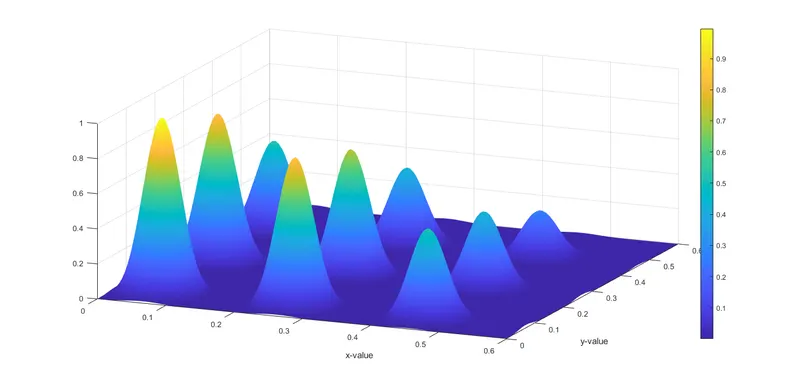
MATLAB program for optimization of a random value and checking the stalagmite function (Unbounded condition or Study-1):

%Start the MATLAB program

clear all

close all

clc

%First of all we need to create one dimensional array

x=linspace(0,0.6,150);

y=linspace(0,0.6,150);

%Now create two dimensional array using meshgrid command

[xx, yy] = meshgrid(x,y);

%Evaluating the Stalagmite Function

for i=1:length(x)

    for j=1:length(y)

        Input_Vector(1) = xx(i,j);

        Input_Vector(2) = yy(i,j);

        f(i,j) = stalagmite_func(Input_Vector);

    end

end

%Iterate 50 times

num_cases =50;

%Study1 (Unbounded)

tic

for i=1:num_cases

    [Input,fmax(i)] = ga(@stalagmite_func,2);

    xopt(i)=Input(1);

    yopt(i)=Input(2);

end

time1=toc;

%Plot the Unbounded graph

figure(1)

subplot(2,1,1)

surfc(x,y,-f)

shading interp

hold on

plot3(xopt,yopt,-fmax,'marker','o','markerfacecolor','r','markersize',6)

title('Unbounded')

subplot(2,1,2)

plot(-fmax)

xlabel('Iteration')

ylabel('fmax')

colorbar()

OUTPUT:

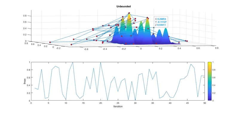
MATLAB program for optimization of a random value and checking the stalagmite function (Bounded condition or Study-2):

%Start the MATLAB program

clear all

close all

clc

%First of all we need to create one dimensional array

x=linspace(0,0.6,150);

y=linspace(0,0.6,150);

%Now create two dimensional array using meshgrid command

[xx, yy] = meshgrid(x,y);

%Evaluating the Stalagmite Function

for i=1:length(x)

    for j=1:length(y)

        Input_Vector(1) = xx(i,j);

        Input_Vector(2) = yy(i,j);

        f(i,j) = stalagmite_func(Input_Vector);

    end

end

%Iterate 50 times

num_cases =50;

%Study 2 (Bounded)

tic

for i=1:num_cases

    [Input,fmax(i)] = ga(@stalagmite_func,2,[],[],[],[],[0;0],[0.6;0.6]);

    xopt(i)=Input(1);

    yopt(i)=Input(2);

end

time2=toc;

%Plotting the Bounded graph

figure(2)

subplot(2,1,1)

surfc(x,y,-f)

shading interp

hold on

plot3(xopt,yopt,-fmax,'marker','o','markerfacecolor','r','markersize',2)

title('Bounded')

subplot(2,1,2)

plot(-fmax)

xlabel('Iteration')

ylabel('fmax')

colorbar()

OUTPUT:

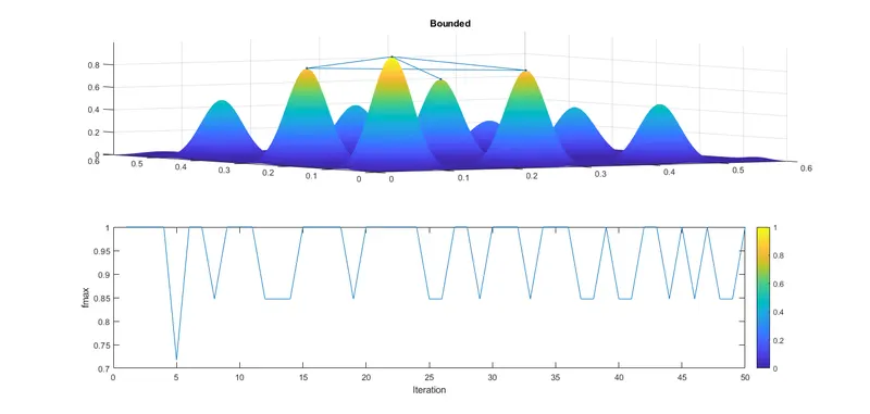
MATLAB program for optimization of a random value and checking the stalagmite function (Bounded condition or Study-3):

%Start the MATLAB program

clear all

close all

clc

%First of all we need to create one dimensional array

x=linspace(0,0.6,150);

y=linspace(0,0.6,150);

%Now create two dimensional array using meshgrid command

[xx, yy] = meshgrid(x,y);

%Evaluating the Stalagmite Function

for i=1:length(x)

    for j=1:length(y)

        Input_Vector(1) = xx(i,j);

        Input_Vector(2) = yy(i,j);

        f(i,j) = stalagmite_func(Input_Vector);

    end

end

%Iterate 50 times

num_cases =50;

%Options

options = optimoptions('ga');

options = optimoptions('ga','Populationsize',250);

%Study 3 (Population bound)

tic

for i=1:num_cases

    [Input,fmax(i)] = ga(@stalagmite_func,2,[],[],[],[],[0;0],[0.6;0.6],[],[],options);

    xopt(i)=Input(1);

    yopt(i)=Input(2);

end

time3=toc;

%Plotting the Population bound graph

figure(3)

subplot(2,1,1)

surfc(x,y,-f)

shading interp

hold on

plot3(xopt,yopt,-fmax,'marker','o','markerfacecolor','r','markersize',2)

title('Population Bound')

subplot(2,1,2)

plot(-fmax)

xlabel('Iteration')

ylabel('fmax')

colorbar()

OUTPUT:

COMBINED MATLAB PROGRAM FOR ALL THREE STUDIES:

%Start the MATLAB program

clear all

close all

clc

%First of all we need to create one dimensional array

x=linspace(0,0.6,150);

y=linspace(0,0.6,150);

%Now create two dimensional array using meshgrid command

[xx, yy] = meshgrid(x,y);

%Evaluating the Stalagmite Function

for i=1:length(x)

    for j=1:length(y)

        Input_Vector(1) = xx(i,j);

        Input_Vector(2) = yy(i,j);

        f(i,j) = stalagmite_func(Input_Vector);

    end

end

%Iterate 50 times

num_cases =50;

%Study1 (Unbounded)

tic

for i=1:num_cases

    [Input,fmax(i)] = ga(@stalagmite_func,2);

    xopt(i)=Input(1);

    yopt(i)=Input(2);

end

time1=toc;

%Plot the Unbounded graph

figure(1)

subplot(2,1,1)

surfc(x,y,-f)

shading interp

hold on

plot3(xopt,yopt,-fmax,'marker','o','markerfacecolor','r','markersize',6)

title('Unbounded')

subplot(2,1,2)

plot(-fmax)

xlabel('Iteration')

ylabel('fmax')

colorbar()

%Study 2 (Bounded)

tic

for i=1:num_cases

    [Input,fmax(i)] = ga(@stalagmite_func,2,[],[],[],[],[0;0],[0.6;0.6]);

    xopt(i)=Input(1);

    yopt(i)=Input(2);

end

time2=toc;

 

%Plotting the Bounded graph

figure(2)

subplot(2,1,1)

surfc(x,y,-f)

shading interp

hold on

plot3(xopt,yopt,-fmax,'marker','o','markerfacecolor','r','markersize',2)

title('Bounded')

subplot(2,1,2)

plot(-fmax)

xlabel('Iteration')

ylabel('fmax')

colorbar()

%Options

options = optimoptions('ga');

options = optimoptions('ga','Populationsize',250);

%Study 3 (Population bound)

tic

for i=1:num_cases

    [Input,fmax(i)] = ga(@stalagmite_func,2,[],[],[],[],[0;0],[0.6;0.6],[],[],options);

    xopt(i)=Input(1);

    yopt(i)=Input(2);

end

time3=toc;

%Plotting the Population bound graph

figure(3)

subplot(2,1,1)

surfc(x,y,-f)

shading interp

hold on

plot3(xopt,yopt,-fmax,'marker','o','markerfacecolor','r','markersize',2)

title('Population Bound')

subplot(2,1,2)

plot(-fmax)

xlabel('Iteration')

ylabel('fmax')

colorbar()

OUTPUT:

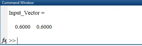
Result: