Solving second order ODEs

Aim: To write a MATLAB program to solve second order ODE for a pendulum and to animate the motion of the pendulum.

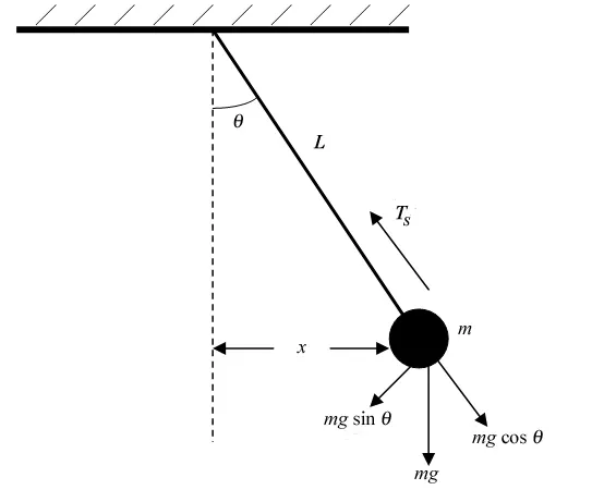
Second Order Differential Equation for a pendulum:

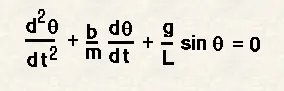
Where,

b is damping coefficient.

m is mass of ball.

g is acceleration due to gravity

l is the length of the string

Assuming,

ϴ = ϴ₁ and dϴ/dt = dϴ₁/dt = ϴ₂

d²ϴ/dt² = d/dt(dϴ₁/dt) = dϴ₂/dt

substituting the above in ODE we get

d² ϴ₂/ dt² + (b/m) ϴ₂ + (g/l)sin ϴ₁ = 0

dϴ₂/dt = ( - (b/m) ϴ₂ - (g/l)sin ϴ₁)

Program:

% Program to solve second order ODE for a pendulum

% Inputs
% Damping coefficient
b = 0.05
% accleration due to Gravity (m/s^2)
g = 9.81
% Length of the string (m)
l = 1
% Mass of the ball (kg)
m = 1

% Initial conditions
theta_0 = [0;3];

% Time
t_span = linspace(0,20,500);

% solving ode
[t, o] = ode45(@(t, theta) ode_function(t, theta, b, g, l, m), t_span, theta_0);

plot(t, o)

Explanation:

. Lines 3 to 14 are the input parameters.

. line 17 specifies the Interval of integration.

. line 20 provides the output [t, result] to plot the graph with the help of an inbuilt ode solver ode45.

. lines 22 to 24 plots the graph from the output values.

Output:

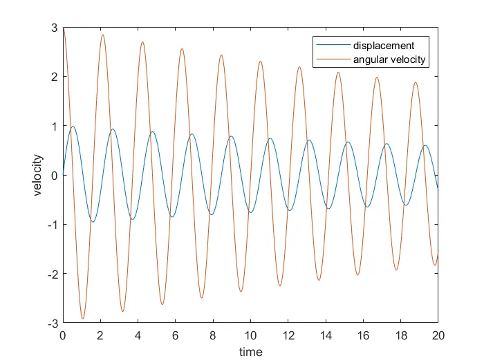
Error:

not specifying the main dependant inputs t, theta due to @ missing in the syntax.

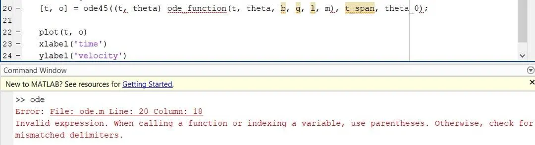
Rectification:

by defining the proper sintax the program gets executed without throwing an error.

Animation to represent the pendulum motion:

Program:

% Program to solve second order ODE for a pendulum

% Inputs
% Damping coefficient
b = 0.05
% accleration due to Gravity (m/s^2)
g = 9.81
% Length of the string (m)
l = 1
% Mass of the ball (kg)
m = 1

% Initial conditions
theta_0 = [0;3];

% Time
t_span = linspace(0,20,500);

% solving ode
[t, o] = ode45(@(t, theta) ode_function(t, theta, b, g, l, m), t_span, theta_0);

% Graph for displacement w.r.t time
plot(t, o(:,1))
hold on
% Graph for velocity w.r.t time
plot(t, o(:,2))
xlabel('time')
ylabel('velocity & displacement')
legend('displacement','angular velocity')
figure;

% Animation

displacement = o(:,1);
ct=1;
for i = 1:length(displacement)
    x0 = 0;
    y0 = 0;
    x1 = l*sin(displacement(i));
    y1 = -l*cos(displacement(i));
    plot([-1 1],[0,0],'linewidth',5)
    hold on
    plot([x0 x1],[y0,y1],'linewidth',3)
    hold on
    plot (x1,y1,'o','MarkerFaceColor','r')
    hold off
    axis([-1.5 1.5 -1.5 1.5])
    pause(0.01)
    M(ct)=getframe(gcf)
    ct=ct+1;
end
  
figure;

% Movie

movie(M)
videofile=VideoWriter('Simple Pendulum.avi','Uncompressed AVI')
open(videofile)
writeVideo(videofile,M)
close(videofile)

Explanation:

. in line 34 we are defining displacement to be used in the for loop and counter value.

. For loop is used to determine the position of the pendulum.

. in i = 1:length(displacement) the value changes each time.

. Lines 37 & 38 fixed points are defined.

. Lines 39 & 40 determines the position of the pendulum.

. Lines 41 to 47 plots the values on the graph.

. Lines 48 to 50 displays the animation for the above plot.

. Lines 57 to 61 creates a video and saves the animation.

Link for the pendulum motion video

https://youtu.be/IlzF-yhXOO0