Week 3 - Solving second order ODEs

In Engineering, ordinary differential equations (ODEs) is used to describe the transient behavior of a system. A simple example is a pendulum

The way the pendulum moves depends on the Newton’s second law. When this law is written down, we get a second order ordinary differential equation that describes the position of the "ball" with respect to time.

Similarly, there are hundreds of ODEs that describe key phenomena and if you have the ability to solve these equations then you will be able to simulate any of these systems.

Your objective is to write a program that solves the following ODE. This ODE represents the equation of motion of a simple pendulum with damping

In the above equation,

g = gravity in m/s2,

L = length of the pendulum in m,

m = mass of the ball in kg,

b = damping coefficient.

Write a program in Python that will simulate the pendulum motion, use; L=1 m, m=1 kg, b=0.05, g=9.81 m/s2.

Simulate the motion between 0-20 sec, for angular displacement=0, angular velocity=3 rad/sec at time t=0.

When you do this you will get the position of the pendulum as a function of time. Use this information to animate the motion of the pendulum.

Aim:

To develop a Python program to solve the second-order ordinary differential equation governing the motion of a damped pendulum, incorporating parameters such as gravity, pendulum length, mass, and damping coefficient. Utilize the solution to simulate the pendulum's motion over a specified time interval and visualize its dynamic behavior through animation.

Objective:

The goal is to create Python code that simulates and animates the movement of a damped simple pendulum using ordinary differential equations. Equations are created to account for damping effects, taking into consideration gravity, length, mass, and damping coefficient. The program uses numerical methods to calculate the angular displacement and velocity of a pendulum over a specified time interval. The software uses matplotlib to create an animation depicting the pendulum's movements. This challenge shows how ODEs can be used in engineering to simulate and depict real-world systems.

Problem Statement:

When illustrating the transient behaviors displayed by different systems, ODEs are widely used in engineering. A pendulum provides a simple example of this principle. The pendulum's motion is based on Newton's second law of motion. Solving the motion equation in Python provides a chance to learn about the scipy library and odeint class. This hands-on method helps understand the necessary parameters for accurate numerical integration and differential equation resolution in this setting. Figure 4 represents the main parameters that need to be considered to characterize the motion of a simple pendulum.

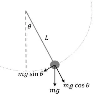
Figure 4: The motion of a simple pendulum.

Equations Used:

The second order differential equation coupled with the arrangement in matrix form:

`(d^2theta)/(dt) + b/m (d theta)/dt + g/l sintheta = 0`

Where,

𝜽 is the angular displacement; 𝒃 is the damping coefficient; 𝒎 is the mass of the bob; 𝒈 is the acceleration due to gravity; 𝒍 is the length of the pendulum

Assuming that `theta = theta_1`and `(d theta_1)/dt = theta_2`, and solving ODE in the matrix form:

`d/dt((theta_1),(theta_2)) = ((theta_2),(-b/mtheta_2 - g/l sintheta_1))`

Program:

import numpy as np
from scipy.integrate import solve_ivp  # Import solve_ivp function
import matplotlib.pyplot as plt
from PIL import Image

# Constants
g = 9.81  # m/s^2
L = 1.0   # m
m = 1.0   # kg
b = 0.05  # damping coefficient

# Function representing the ODE
def pendulum_ode(t, y):
    theta, omega = y
    dydt = [omega, -(b/m) * omega - (g/L) * np.sin(theta)]
    return dydt

# Initial conditions
theta_0 = 0.0  # initial angular displacement
omega_0 = 3.0  # initial angular velocity

# Time span
t_span = (0, 20)  # from 0 to 20 seconds

# Solve ODE
sol = solve_ivp(pendulum_ode, t_span, [theta_0, omega_0], t_eval=np.linspace(0, 20, 500))

# Extract results
t = sol.t
theta = sol.y[0]
omega = sol.y[1]

# Plot Time vs Angular Displacement and Angular Velocity
plt.figure(figsize=(10, 6))
plt.plot(t, theta, label='Angular Displacement')
plt.plot(t, omega, label='Angular Velocity')
plt.title('Time vs Angular Displacement and Angular Velocity')
plt.xlabel('Time (s)')
plt.ylabel('Value')
plt.legend()
plt.grid(True)
plt.show()

# Create frames for the animation
frames = []
for i, angle in enumerate(theta):
    x1, y1 = 0, 0
    x2, y2 = L * np.sin(angle), -L * np.cos(angle)

    plt.figure()
    plt.plot([-2.0, 2.0], [0, 0], 'y', linewidth=5)
    plt.plot([x1, x2], [y1, y2], linewidth=3)
    plt.plot(x2, y2, 'o', markersize=20, markerfacecolor='w')
    plt.plot(x1, y1, 'o', markersize=10, markerfacecolor='r')
    plt.xlim([-2.0, 2.0])
    plt.ylim([-2.0, 0.5])

    filename = f"frame_{i}.png"
    plt.savefig(filename)
    plt.close()

    frames.append(Image.open(filename))

# Save frames as a GIF
frames[0].save('Simple_Pendulum.gif', format='GIF', append_images=frames[1:], save_all=True, duration=60, loop=0)

Explanation:

The provided code simulates and visualizes the motion of a simple pendulum using numerical integration techniques. Here's a detailed explanation of each part:

Importing Libraries:

import numpy as np
from scipy.integrate import solve_ivp
import matplotlib.pyplot as plt
from PIL import Image

This block imports necessary libraries:

• numpy for numerical computing.
• solve_ivp from scipy.integrate for solving initial value problems.
• matplotlib.pyplot for plotting.
• Image from PIL (Python Imaging Library) for working with images.

Defining Constants:

g = 9.81  # m/s^2
L = 1.0   # m
m = 1.0   # kg
b = 0.05  # damping coefficient

Defines physical constants for the pendulum system: acceleration due to gravity (g), length of the pendulum (L), mass of the pendulum (m), and damping coefficient (b).

Defining the ODE function:

def pendulum_ode(t, y):
    theta, omega = y
    dydt = [omega, -(b/m) * omega - (g/L) * np.sin(theta)]
    return dydt

• Defines the Ordinary Differential Equation (ODE) function for the simple pendulum.
• The function takes time t and a vector y containing the angular displacement theta and angular velocity omega.
• Returns the derivatives of theta and omega.

Setting Initial Conditions:

theta_0 = 0.0  # initial angular displacement
omega_0 = 3.0  # initial angular velocity

Sets initial conditions for the pendulum: initial angular displacement (theta_0) and initial angular velocity (omega_0).

Defining Time Span:

t_span = (0, 20)  # from 0 to 20 seconds

Defines the time span for which the simulation will be run.

Solving the ODE:

sol = solve_ivp(pendulum_ode, t_span, [theta_0, omega_0], t_eval=np.linspace(0, 20, 500))

• Solves the ODE using solve_ivp function.
• Passes the ODE function, time span, initial conditions, and specifies the times at which to evaluate the solution.

Extracting Results:

t = sol.t
theta = sol.y[0]
omega = sol.y[1]

Extracts time (t), angular displacement (theta), and angular velocity (omega) from the solution.

Plotting Time vs Angular Displacement and Angular Velocity:

plt.figure(figsize=(10, 6))
plt.plot(t, theta, label='Angular Displacement')
plt.plot(t, omega, label='Angular Velocity')
plt.title('Time vs Angular Displacement and Angular Velocity')
plt.xlabel('Time (s)')
plt.ylabel('Value')
plt.legend()
plt.grid(True)
plt.show()

Plots time vs angular displacement and angular velocity.

Creating Frames for Animation:

frames = []
for i, angle in enumerate(theta):
    x1, y1 = 0, 0
    x2, y2 = L * np.sin(angle), -L * np.cos(angle)

    plt.figure()
    plt.plot([-2.0, 2.0], [0, 0], 'y', linewidth=5)
    plt.plot([x1, x2], [y1, y2], linewidth=3)
    plt.plot(x2, y2, 'o', markersize=20, markerfacecolor='w')
    plt.plot(x1, y1, 'o', markersize=10, markerfacecolor='r')
    plt.xlim([-2.0, 2.0])
    plt.ylim([-2.0, 0.5])

    filename = f"frame_{i}.png"
    plt.savefig(filename)
    plt.close()

    frames.append(Image.open(filename))

• Creates frames for the animation by iterating over the angular displacements.
• Plots the pendulum at each angle and saves the plot as an image.
• Appends each image to the frames list.

Saving Frames as a GIF:

frames[0].save('Simple_Pendulum.gif', format='GIF', append_images=frames[1:], save_all=True, duration=60, loop=0)

• Saves the frames as a GIF animation.
• Uses the first frame as a reference and appends other frames to it.
• Specifies the duration for each frame and sets the loop count to infinite.

Output:

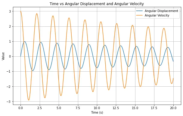
Time vs Angular Displacement and Velocity

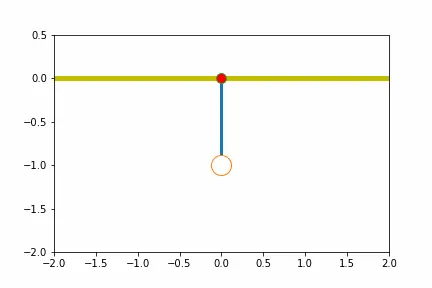
Simple Pendulum Animation

The plot generated offers a comprehensive visualization of a damped simple pendulum's angular displacement and angular velocity within a specified time frame. The blue line portrays the pendulum's angular displacement changes, showcasing its oscillatory motion around the equilibrium point. Angular velocity is represented by the orange line, reflecting the pendulum's rotation speed across different time intervals. Clearly labeled axes provide contextual information, with time on the horizontal axis and angular displacement/velocity on the vertical axis. A legend differentiates between the two lines, while the title "Angular Displacement and Velocity of Simple Pendulum" concisely summarizes the plot's essence. The presence of a grid enhances precision in reading values. Altogether, the plot adeptly captures the dynamic interplay between angular displacement and angular velocity as the pendulum's motion unfolds over time.

Extras:

I have attached another ZIP file (Simple Pendulum with Damping) with the same code of the original zip file (Simple Pendulum), but the parameter of damping co-efficient is changed to "b = 0.5".

By changing the damping coefficient to "b = 0.5", the damping effect increases. This means that the pendulum experiences a stronger resistance against its motion, leading to quicker dissipation of its energy.