Week 3 - Solving second order ODEs

AIM:

• To create an animation of simple pendulum by using second order differential equation by using ode solver function.
• For simulation the second order equation of the simple pendulum is:
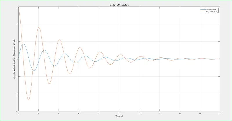
• To create a plot between angular velocity and displacement of simple pendulum by using ode45.

CONCEPT:

• For a simple pendulum with a damping factor, the equation of simple pendulum is

Where

b = damping coefficient (N-m/s)

m = mass of the bob (kg)

g = gravitational acceleration (m/s)

l = length of the string to connect bob (m)

• The above equation is having a differential power of order 2. To use ode45 solver which is developed on the basis of RK method which uses the simple differential equation to solve the higher order differential equations.

OBJECTIVE:

• By using ode45 solver which is an inbuilt solver in the MATLAB. The ode45 solver should require simple differential equation to solve any kind of higher order differential equation.
• By taking constants we can solve the higher order differential equation to a simple ordinary differential equation.

Let us consider

θ = θ1 ------ (1)

dθ/dt = dθ₁/dt = θ₂ ------(2)

d²θ/dt² = dθ₂/dt -------(3)

• By using these constants, the second order equation will become as:

dθ₂/dt = -(b/m) * θ₂ – (g/l) * sinθ

• The simple differential equations are written in the form of a matrix

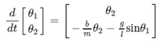
• By using the above equation and the ode45 solver we can animate the simple pendulum in the MATLAB by writing a code.

Code:

% program for simple pendulum using ode45.
clear theta1 theta2 dtheta1_dt dtheta2_dt
close all
clc

% input variables for the second-order ODE of a simple pendulum
b = 0.05;
g = 9.81;
l = 1;
m = 0.1;

theta_0 = [0; 3];

t_span = linspace(0, 20, 500);

% ode45 function to solve second-order ODE
[t, results] = ode45(@(t,theta) ode_func(t,theta,b,g,l,m), t_span, theta_0 );

% plotting of angular velocity and displacement
figure(1)
plot(t, results(:,1))
hold on
plot(t, results(:,2))
grid on
title('Motion of Pendulum')
xlabel('Time (s)')
ylabel('Angular Velocity (rad/s) / Displacement (rad)')
legend('Displacement','Angular Velocity')

angle = results(:,1);

% count command for iterations.
ct = 1;

% Create a folder to store the PNG images
foldername = 'pendulum_frames';
if ~exist(foldername, 'dir')
    mkdir(foldername);
end

for i = 1 : length(angle)
    omega = angle(i);
    figure(2)
    title('Motion of Pendulum')
    
    % fixed coordinates of one end of the simple pendulum.
    x0 = 0;
    y0 = 0;
    
    % moving coordinates of the bob.
    x1 = l*cos((3*pi/2)+omega);
    y1 = l*sin((3*pi/2)+omega);
    
    % plotting of the bob motion.
    plot([x0 x1],[y0 y1],'linewidth',3,'color','g');
    hold on;
    plot(x1,y1,'o','MarkerSize',15,'MarkerFaceColor','k');
    hold on;
    plot([-3 3],[0 0],'linewidth',2,'color','b','MarkerSize',15);
    hold off
    axis([-3 3 -2 2])
    grid on 
    pause(0.1)
    M(ct) = getframe(gcf);
    
    % Save each frame as a PNG image
    framefilename = sprintf('%s/frame_%04d.png', foldername, ct);
    imwrite(M(ct).cdata, framefilename);
    
    ct = ct + 1;
end

% Use imageio library in Python to convert the PNG images into a GIF file
system(sprintf('python -m imageio.plugins.ffmpeg.download --path "%s"', matlabroot));  % Download imageio FFMpeg plugin if needed
system(sprintf('python -m imageio --output "%s/pendulum_animation.gif" "%s/*.png"', foldername, foldername));  % Convert PNG images to GIF

function [dtheta_dt] = ode_func(t,theta,b,g,l,m)
    theta1 = theta(1);
    theta2 = theta(2);
    dtheta1_dt = theta(2);
    dtheta2_dt = -(b/m)*theta2 - (g/l)*sin(theta1);
    dtheta_dt = [dtheta1_dt; dtheta2_dt];
end

Explanation Of this Code:

Certainly! Here's a step-by-step explanation of the modified code with detailed explanations and commands:

1. The initial part of the code clears some variables and closes any open figures, providing a clean workspace to work with.

2. The input variables `b`, `g`, `l`, and `m` are defined for the second-order ODE that represents the simple pendulum.

3. The initial conditions `theta_0` and the time span `t_span` are set for the simulation.

4. The `ode45` function is used to solve the second-order ODE by calling the `ode_func` function, which defines the equations of motion for the simple pendulum. The solution is obtained in the variables `t` and `results`.

5. A new figure (`figure(1)`) is created for plotting the angular velocity and displacement of the pendulum using `plot` commands.

6. The angles (`angle`) are extracted from the `results` variable.

7. A counter variable `ct` is initialized to keep track of the iterations.

8. A folder named `'pendulum_frames'` is created to store the individual frames of the animation. If the folder already exists, the `mkdir` command will not create it again.

9. A loop is used to iterate over each angle in the `angle` variable.

10. Inside the loop, the moving coordinates of the pendulum bob are calculated based on the current angle (`omega`).

11. The motion of the pendulum is visualized by plotting the pendulum and the bob using `plot` commands.

12. The animation is paused for 0.1 seconds using the `pause` command to control the speed of the animation.

13. The current frame is captured using `M(ct) = getframe(gcf)` and saved as a PNG image using the `imwrite` command. The frame is saved with a file name in the format `frame_####.png`, where `####` represents a four-digit frame number.

14. The counter `ct` is incremented for the next iteration.

15. After the loop finishes, the MATLAB script calls Python using the `system` command to convert the PNG images in the `'pendulum_frames'` folder into a GIF file. The Python code uses the `imageio` library to convert the images. Note that the `imageio` library needs to be installed in your Python environment.

16. The `ode_func` function defines the ODE equations for the simple pendulum. It takes the time `t`, the current state vector `theta`, and the parameters `b`, `g`, `l`, and `m`. The function calculates the derivatives of `theta` and returns them in `dtheta_dt`.

That's a detailed explanation of the code. It simulates the motion of a simple pendulum, saves individual frames as PNG images, and then converts them into a GIF file using Python's `imageio` library.

Output Plot:

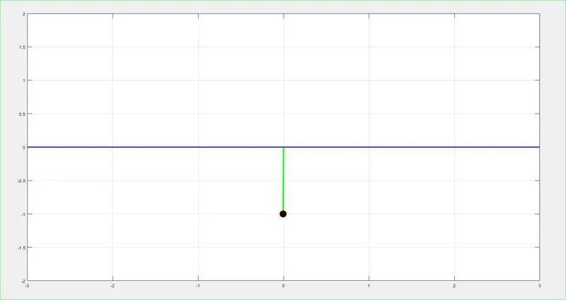
Note: GIF Animation Uploded on the Drive Files.

Wave Plot:

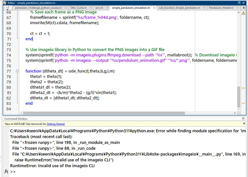
Error faced:

CONCLUSION:

• We have animated the simple pendulum using the ode45 solver where the second order is reduced to a simple differential equation where it is easy to solve the given equation.
• The animation is made using the different points of the bob and the motion of the simple pendulum is created.

Drive Link:

https://drive.google.com/drive/folders/1-A4dYyzlzFzlDeeRtmjO840Be-mCPvcl?usp=drive_link

Youtube Link:

https://youtu.be/mSH-Jyi2m3M