Week 3 - Solving second order ODEs

Objective:

Write a program to simulate the transient behavior of a simple pendulum and create an animation of it\'s motion.

Theory: A function was defined for calculating the angular displacement and velocity of the simple pendulum at different time intervals. The second-order differential equation defining the motion of the pendulum

`(d^2 θ)/ (d t^2) + b/m . (dθ)/(dt) + g/l . sin θ = 0

where, b = damping.

m = mass.

g = gravity.

l = length.

Code:

#Program to describe the transient behavior of a simple pendulum


import numpy as np 
from scipy.integrate import odeint
import matplotlib.pyplot as plt
import math


#funcion that returns dtheta/dt

def model(theta,t,b,g,l,m):
	theta1 = theta[0]
	theta2 = theta[1]
	dtheta1_dt = theta2
	dtheta2_dt = -(b/m)*theta2-(g/l)*math.sin(theta1)
	dtheta_dt = [dtheta1_dt,dtheta2_dt]
	return dtheta_dt

#Inputs parameters
b=0.05 # Damping Coefficient 
g=9.81 #Gravity in m/s^2
l=1 # Length in metre
m=1 # MAss in Kg 

#initial condition

theta_0 = [0,5]

#time points 
t = np.linspace(0,10,150)

#solve ODE

theta  = odeint(model,theta_0,t,args = (b,g,l,m))


#plot results

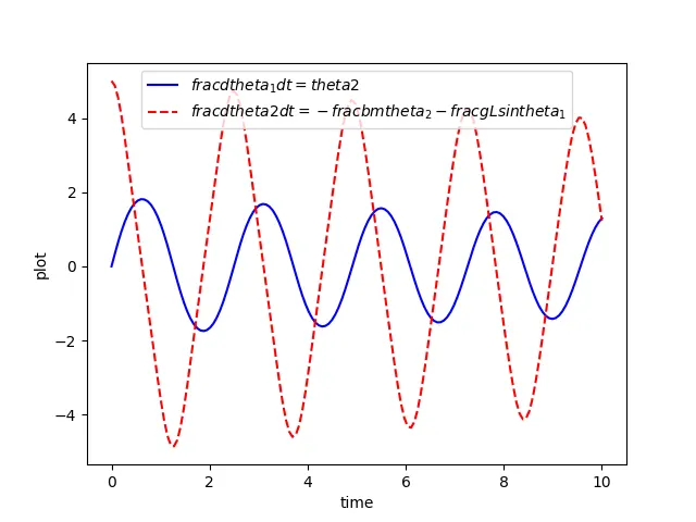
plt.plot(t,theta[:,0],'b-',label=r'$frac{dtheta_1}{dt}=theta2$')
plt.plot(t,theta[:,1],'r--',label=r'$frac{dtheta2}{dt}=-frac{b}{m}theta_2-frac{g}{L}sintheta_1$')
plt.ylabel('plot')
plt.xlabel('time')
plt.legend()
plt.savefig('Output.png')
plt.show()

#animation program
ct = 1

x0 = 0
y0 = 0

for i in theta[:,0]:
	
	x1 = (1*math.sin(i))
	y1 = (-1*math.cos(i))

	filename = str(ct) + '.png'
	ct = ct +1
	
	plt.figure()
	plt.plot([-1,1],[0,0],"black",linewidth=10)
	plt.plot([x0,x1],[y0,y1],"red")
	plt.plot(x1,y1,'o',markersize = 20)
	plt.xlim([-1.5,1.5])
	plt.ylim([-1.5,1.0])
	plt.savefig(filename)

Code Explanation:

• Import module numpy as np, scipy.intedrate import odeint for second ODE, math and for plots matplotlib.
• Break down the second-order ODE into two first-order ODE, the first ode will give the values of displacement and second ODE will give the values of velocity.
• Defining 1st-order order ODEs.
• Passing initial values and initial conditions for theta1 & theta2.
• To obtain smooth motion create an array of times using linspace command.
• Solving ODE using odeint by calling defined ODE’s.
• Plotting Angular displacement and Velocity Vs Time.
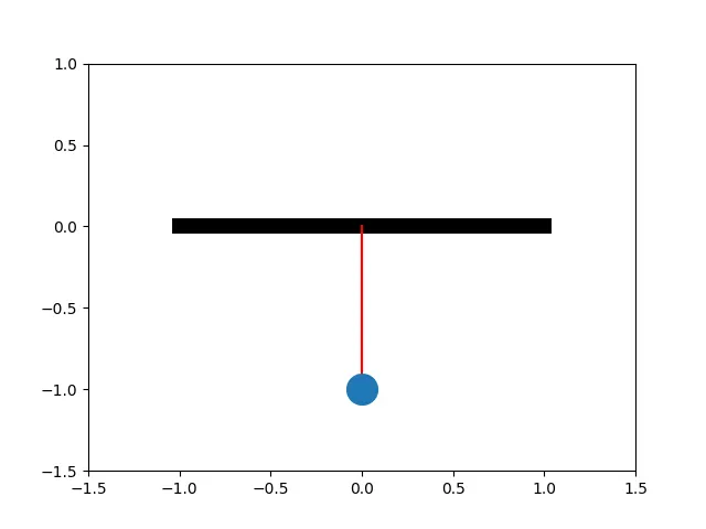
• Plotting state of simple pendulum on Graph and saving images.
• Sewing all images together to create GIF of simple pendulum motion.

Results:

Animated GIF:

Animated Video:

https://youtu.be/XfJeC9n1utU