Week 3 - Solving second order ODEs

AIM :

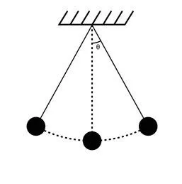
In Engineering, ODE is used to describe the transient behavior of a system. A simple example is a pendulum

The way the pendulum moves depends on the Newtons second law. When this law is written down, we get a second order Ordinary Differential Equation that describes the position of the "ball" w.r.t time.

Similarly, there are hundreds of ODEs that describe key phenomena and if you have the ability to solve these equations then you will be able to simulate any of theses systems.

Your objective is to write a program that solves the following ODE. This ODE represents the equation of motion of a simple pendulum with damping

Theory: A function was defined for calculating the angular displacement and velocity of simple pendulum at different time intervals. The second-order differential equation defining the motion of pendulum

In the above equation,

g = gravity in m/s2,

L = length of the pendulum in m,

m = mass of the ball in kg,

b=damping coefficient.

Write a program in Python that will simulate the pendulum motion, just like the one shown in the start of this challenge.

use,

L=1 metre,

m=1 kg,

b=0.05.

g=9.81 m/s2.

Simulate the motion between 0-20 sec, for angular displacement=0,angular velocity=3 rad/sec at time t=0.

When you do this you will get the position of the pendulum as a function of time. Use this information to animate the motion of the pendulum, as shown in the below figure.

Procedure:

• Importing math,matplotlib,numpy,image,glob libraries
• Defining 1^st order ODE’s .
• Passing initial values.
  1. b = 0.5
  2. g = 9.81
  3. l = 1
  4. m = 1
• Passing initial condition for theta1 & theta2.
• Passing (t) for 20 sec and dividing it into 200 times.
• Solving ODE using odeint by calling defined ODE’s.
• Plotting Angular displacement and Velocity Vs Time.
• Plotting state of simple pendulum on Graph and saving images.
• Sewing all images together to create GIF of simple pendulum motion.

The second order differential equation used for a simple pendulum is as following -

d2θdt2+bmdθdt+gLsinθ=0d2θdt2+bmdθdt+gLsin⁡θ=0 (i)

Where,

b = damping coefficient = 0.05 Ns/m;

m = mass of bob = 0.1 kg;

g = gravitation acceleration = 9.81 m/s²;

L = length of the string = 1 m;

Above differential equation can be solved if we convert it into a first order differential equation.

Let, θ=θ1θ=θ1 (ii)

and, dθ1dt=θ2dθ1dt=θ2 (ііi)

then, d2θ1dt2=ddt(dθ1dt)=dθ2dtd2θ1dt2=ddt(dθ1dt)=dθ2dt (iv)

so the eq. (i) becomes,

dθ2dt=−bmθ2−gLsinθ1dθ2dt=-bmθ2-gLsinθ1 (v)

hence eq. (iii) and eq. (v) can be written as a matrix of dθdtdθdt.

ddt[θ1,θ2]=[θ2,−bmθ2−gLsinθ1]

PROGRAM GENERATED FROM PYTHON :

# To solve 2nd order ODE using python

import numpy as np 
from scipy.integrate import odeint
import math
import matplotlib.pyplot as plt

#function that returns dtheta/dt

def function(theta,t,b,g,l,m):
	theta1 = theta[0]
	theta2 = theta[1]
	dtheta1_dt = theta2
	dtheta2_dt = -(b/m)*theta2-(g/l)*math.sin(theta1)
	dtheta_dt = [dtheta1_dt,dtheta2_dt]
	return dtheta_dt


b=0.5
g=9.81
l=1
m=1

# initial conditions
theta_0 = [0,3]

# input for time
t = np.linspace(0,20,200)

theta = odeint(function,theta_0,t,args=(b,g,l,m))

#plot result
plt.plot(t,theta[:,0],'-g',label = r'$\frac{d\theta_1}{dt}=\theta2$')
plt.plot(t,theta[:,1],'b--',label=r'$\frac{d\theta2}{dt}=-\frac{b}{m}\theta_2-\frac{g}{1}sin\theta_1$')
plt.xlabel('Plot')
plt.ylabel('Time')
plt.legend()
plt.savefig('output.png')
plt.show()

# To create Animation
ct = 1
x0 = 0 
y0 = 0

for i in theta[:,0]:
	x1=x0+(1*math.sin(i))
	y1=y0+(-1*math.cos(i))

	filename = str(ct)+'.png'
	ct = ct+1

	plt.figure()
	plt.plot([-1,1],[0,0],"black")
	plt.plot([x0,x1],[y0,y1],"red")
	plt.plot(x1,y1,'o',markersize = '20')
	plt.xlim([-1.5,1.5])
	plt.ylim([-1.5,1.0])
	plt.savefig(filename)
	plt.plot()

STEPWISE EXPLANATION OF THE PROGRAM :

The first part of this about importing the diffferent libraries. Thus, the "numpy" library is imported as np and from "scipy.integrate" the "odeint" library is imported for integration. The "matplotlib.pyplot" library is also imported as plt and the "math" module is also imported.

After that comes the second part of the program which is about the function definition. The function "model" is defined which let us compute the first and second ODE staated above under equation session. The next part is about the definition of input variables. The damping coefficient, gravity, the pendulum length, the displacement and velocity, time as well as the mass are defined. Then the "odeint" library is called to integrate the "model" function.

The fourth part of the program deal with plotting the two simplified ODEs using "plt" and 'plot' command. Plotting is done and legend is shown using 'legend' command.

In the fifth part of this program, the code deals with the creation of pendulum anaimation. The initial position of the pendulum rod is defined; then a counter is also defined which will let us create and store each image corresponding to each position of the pendulum. Under a for loop, each position of the pendulum is computed and stored as an image; those images which will be stiched together to give a full animation. After that, the pendulum is ploted using "markersize" command to create the mass at the end of the pendulum rod. A title is given to the plot using "title" command.

This marks the end of our program.

PLOT GENERATED FROM RUNNING THE CODE :

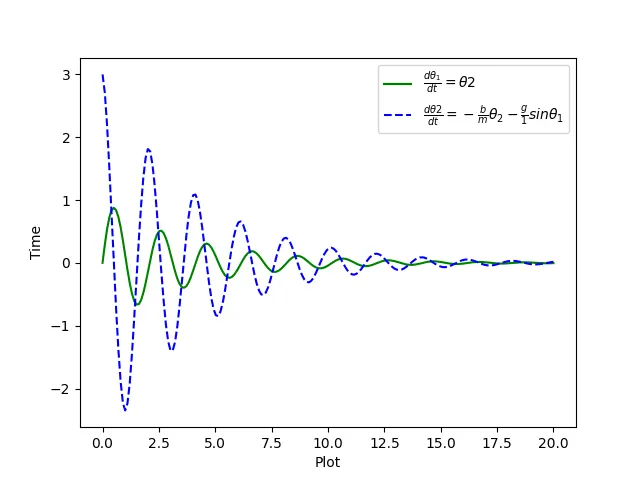
The above plot is generated from running the program.

ERRORS :

The above error is occured due to insuficient command of storing of the images.

The above error is eliminated by using the ''plt.plot()''

CONCLUSION : We have established and created the simulation of motion of simple pendulum by solving the given second order ODE.

The simulation of simple pendulum motion can be consulted through the below: