Week 3 - Solving second order ODEs

AIM:

To Write a program in Matlab\Octave that will simulate the pendulum motion and to animate it.

OBJECTIVES:

• To write a program that solves the following ODE.
• To animate the motion of the pendulum

INTRODUCTION:

• SIMPLE PENDULUM:

A heavy point mass suspended by a weightless, perfectly flexible and inextensible string, from a perfectly rigid support is called “SIMPLE PENDULUM”.

The tension in the string depends both on mg and centripetal force

`(mv^2)/l`

The acceleration of the simple pendulum will be given by,

a=-gsin⁡θ">a=−gsinθa=-gsin⁡θ

The time period of the simple pendulum is,

T=2πω">T=2*π/ω

• WHAT IS ODE?

An ordinary differential equation is an equation containing an unknown function of one real or complex variable x. The unknown function is generally represented by a variable which therefore depends on x.

`(d y) /(d x) = F ( x )`

In engineering, ODE is used to describe the transient behaviour of a system. A example is a simple pendulum. The following is the second order ode of a simple pendulum. The way the pendulum moves depends on the newtons second law .

Newtons second law of motion states that the acceleration of the object is directly proportional to the net force acting on it, and inversely proportional to its mass. When this law is written in differential equations we will get the ordinary differential equation.

The second-order ode for simple pendulum is represented as,

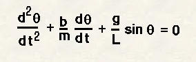
where; b = damping coefficient 0.03,

m = mass of ball 0.8 kg,

g = acceleration due to gravity 9.81 m/s^2,

l = length of the string 1 metre.

Here in MATLAB, we solve ODE by converting into matrix form.calculation for that is shown below;

assume θ=θ1

`(dθ)/dt=(dθ1)/dt=θ2`−−−−[1]

`(d^2θ)/dt^2=(d^2θ1)/dt^2=d/dt((dθ1)/dt)=d(θ2)`−−−−[2]

Now

`(d^2θ)/dt^2+b/m.(dθ)/dt+g/l*(sinθ)`=0

put θ=θ1

`(d^2θ1)/dt^2+b/m.(dθ1)/dt+g/l*(sinθ1)`=0

put θ1=θ2

`(dθ2)/dt+b/m.(θ2)+g/l*(sinθ1)`=0

finally we get ;

`(dθ1)/dt=θ2`

`(dθ2)/dt=−b/mθ2−g/l*(sinθ1)`

In matrix

`d/dt[[θ1],[θ2]]`= `[[θ2],[−b/m(θ2)−g/l(sinθ1)]]`

by solving these we will get the θ1">θ1 and θ2">θ2 values of the simple pendulum.

MATLAB CODE AND ITS EXPLANATION OF THE CODE:

STEP 1 : by using a function command

function [dtheta_dt] = ode_function(t,theta,b,g,l,m)
         theta1 = theta(1)
         theta2 = theta(2)
         dtheta1_dt = theta2;
         dtheta2_dt = -(b/m)*theta2-(g/l)*sin(theta1);
         dtheta_dt = [dtheta1_dt; dtheta2_dt];
         
end

STEP 2: Setting initial values

The initial conditions for solving the ode are,

lengthof the string l = 1m,

mass of the bob, m = 1kg,

damping coefficient,b = 0.05,

acceleration due to gravity, g = 9.81.

% Inputs 
% Damping coefficient
b = 0.05;

% Acceleraton due to gravity
g = 9.81;

% Mass of the ball
m = 1;

%Length of the string
l = 1;

% Initial condition 
theta_0 = [0;5];

% Timepoints
t_span = linspace(0,20,500);

STEP 3 : use of for loop , lin space command and some general commands

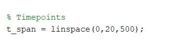
Linspace:

In linsapce command the first value represents the starting point of angle, similarly, the second point represents the ending point of the angle and at last, the third point represents the number of values between them

for-loop:

A for loop is a repetition control structure that allows you to efficiently write a loop that needs to execute a specific number of times.

for i = 1:length(theta2)
    theta3 = theta2(i);
    
    x0 = 0;
    y0 = 0;
    
    x1 = l*sin(theta3);
    y1 = -l*cos(theta3);
   
    figure(3)
    plot([-1.1 1.1],[0 0],'linewidth',2);
    hold on
    plot([x0 x1],[y0 y1],'color','r','linewidth',2)
    hold on
    plot(x1,y1,'o','markers',20,'markerfacecolor','b')
    hold off 
    grid on 
    axis([-1.5 1.5 -1.5 0.5])
    pause(0.03)
    M(ct) = getframe(gcf);
    ct = ct+1;
    
end

legends:

legend creates a legend with descriptive labels for each plotted data series. For the labels, the legend uses the text from the DisplayName properties of the data series. If the DisplayName property is empty, then the legend uses a label of the form 'dataN' .

ode45:

ode45 is a versatile ODE solver and is the first solver you should try for most problems. However, if the problem is stiff or requires high accuracy, then there are other ODE solvers that might be better suited to the problem.'

markers:

Adding markers to a line plot can be a useful way to distinguish multiple lines or to highlight particular data points.

markerfacecolor:

it's also doable to just choose whatever predefined color as when choosing what your marker color is.

STEP 4 : creating animation of the simple pendulum

To create movie type M(ct)=getframe(gcf) just below the pause(0.03) and at extreme end command type movie(M)

Where:-

ct represents every frame and getframe command represents to getting the current figure in the gcf window. Further, we are going to save all the figures in the array called (M).

FINAL CODING IS AS FOLLOWS:

clear all 
close all
clc

% Inputs 
% Damping coefficient
b = 0.05;

% Acceleraton due to gravity
g = 9.81;

% Mass of the ball
m = 1;

%Length of the string
l = 1;

% Initial condition 
theta_0 = [0;5];

% Timepoints
t_span = linspace(0,20,500);

% Solving ode 
[t,results] = ode45(@(t,theta) ode_function(t,theta,b,g,l,m),t_span,theta_0);

% Plotting 
figure(1)
plot(t,results(:,1),'linewidth',1)
hold on 
grid on
plot(t,results(:,2),'linewidth',1)
axis([0 20 -5 5])
xlabel('Time - sec')
ylabel('Angular Velocity & Displacement')
legend('change in displacement','change in angular velocity')
hold off

figure(2)
plot(results(:,1),results(:,2))
grid on
xlabel('Position - rad')
ylabel('Angular Velocity - rad/sec')


theta2 = results(:,1);
ct = 1;
for i = 1:length(theta2)
    theta3 = theta2(i);
    
    x0 = 0;
    y0 = 0;
    
    x1 = l*sin(theta3);
    y1 = -l*cos(theta3);
   
    figure(3)
    plot([-1.1 1.1],[0 0],'linewidth',2);
    hold on
    plot([x0 x1],[y0 y1],'color','r','linewidth',2)
    hold on
    plot(x1,y1,'o','markers',20,'markerfacecolor','b')
    hold off 
    grid on 
    axis([-1.5 1.5 -1.5 0.5])
    pause(0.03)
    M(ct) = getframe(gcf);
    ct = ct+1;
    
end
movie(M)
videofile = VideoWriter('simplependulum.avi','Uncompressed AVI');
open(videofile)
writeVideo(videofile,M)
close(videofile)

RESULT:

thus these are the plots obtained for the above coding

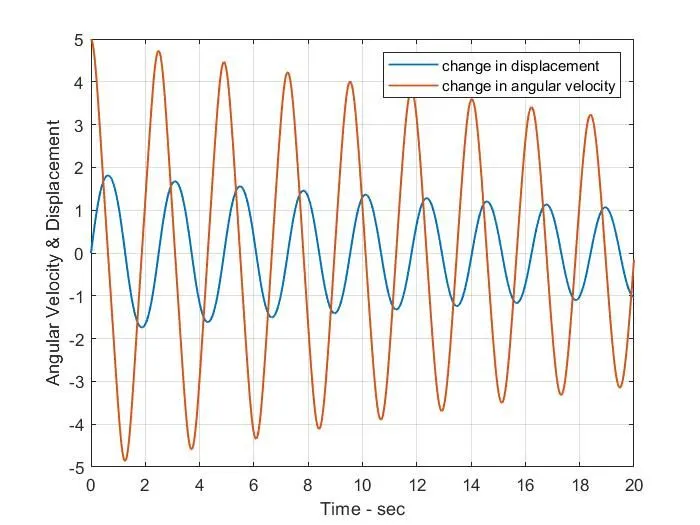
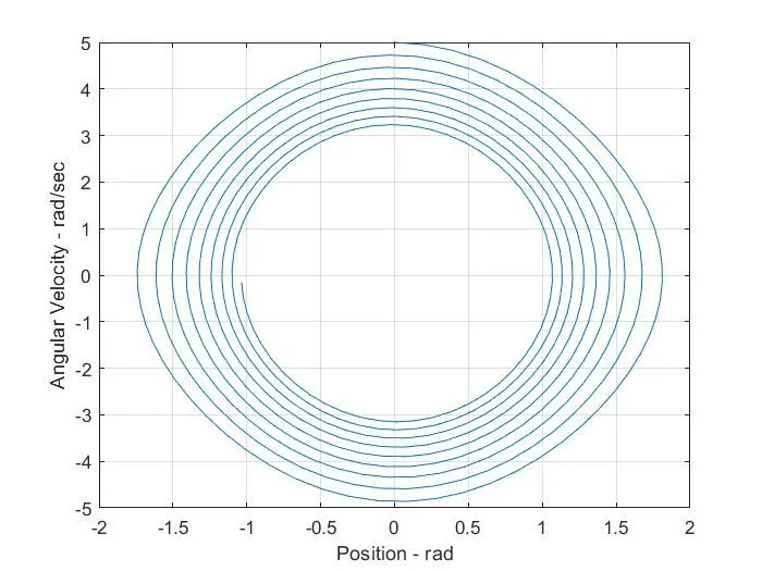
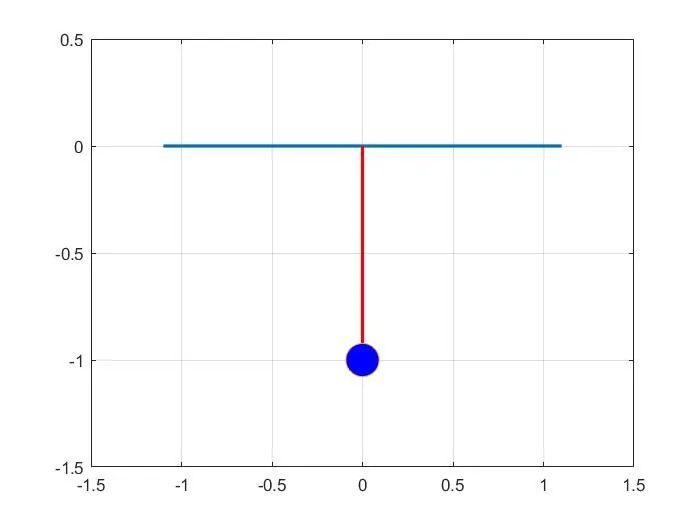
the animation video link is given below

https://youtu.be/yUK8shgKVyA

Errors faced while writing the code:

adding the hold off was neccessary so that new plots added to the axes clear existing plots and reset all axes properties.before that i was not able get output in desired manner.

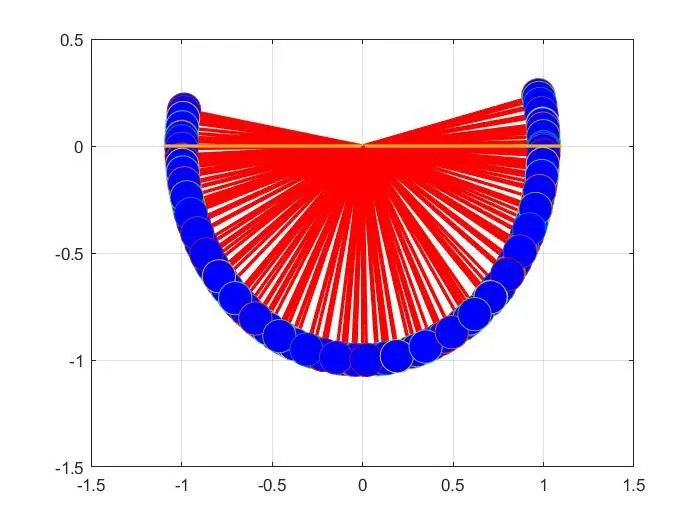
this was my output before the hold off command being added.

my other eroor is the above one i used small m in the above command it gets added with the mass that i have mentioned with small m too so i have changed that into capital M and the issue has been resolved.

CONCLUSION:

thus we have obtained the desired output. we can change the values to get different outputs based on our requirements