Week 3 - Solving second order ODEs

Aim:

Solving a second order ordinary differential equation of simple pendulum and showing the effect of damping by an animation.

Objective:

• To convert second order ordinary differential equation to 1st order ordinary differential equation.
• To create the function using MATLAB in-built function for solving ordinary differential equation.
• To plot the displacement and velocity damping through the time stipulated time of simulation.
• To make the animation of simple pendulum.

Code Explanation:

• the inputs are provided in the problems. Then we make time domain for which the whole code is going to run using the ‘linspace’ command from 0 to 20 seconds with 100 value in between them.
• we provide the initial condition for the angular displacement and velocity which is column vector form, because we need to calculate both value from the equation of motion for plotting purpose.
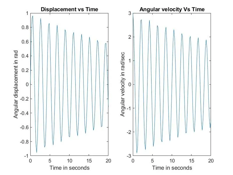
• plotting is done in which subplot command is used, in the first plot first column is plotted and in second subplot second column is plotted with respect to time
• Then we have created a for loop for which we are creating the frame motion for the simple pendulum and saved in the movie.

Code:

clear all
close all
clc

b = 0.05;   
g = 9.81;   
l = 1;      
m = 1;

t_span = linspace(0,20,100);
y_initial = [0;3];

a = @(t,y)ode_second_order_pendulum(y,b,m,l,g);
[t,y]= ode45(a,t_span,y_initial);

figure(1);
grid on
subplot(1,2,1)
plot(t,y(:,1));
title('Displacement vs Time');
xlabel('Time in seconds');
ylabel('Angular displacement in rad');
subplot(1,2,2)
plot(t,y(:,2));
title('Angular velocity Vs Time')
xlabel('Time in seconds');
ylabel('Angular velocity in rad/sec');
grid off
saveas(figure(1),'subplot','jpg')

y1 = -1*cos(y(:,1));
x1 = 1*sin(y(:,1));

for i = 1:100
    figure(2)
    plot([0 x1(i)],[0 y1(i)],'linewidth',3,'color','r');
    hold on
    plot(x1(i),y1(i),'marker','o','linewidth',10,'markerfacecolor','g');
    plot([-1.2 1.2],[0 0],'linewidth',3,'color','b');
    axis([-1.2 1.2 -1.2 1.2]);
    title(['Time: ', num2str(t_span(i))]);
    M(i) = getframe(gcf);
    close(2)
end

movie(M)
videofile = VideoWriter('singlependulum.avi','Uncompressed AVI');
open(videofile);
writeVideo(videofile,M)
close(videofile)

we can see from the plots that the displacement is getting reduced as we move further in to time because of damping factor. we can observe displacement is starting from 0 as initial condition. In the angular velocity vs time plot it has started from 3 rad/sec and then further get decrease.

Video Link:

https://drive.google.com/file/d/1Wu-pdDnhzO1RJAO-e7fNXFwxdc2UXuBm/view?usp=sharing

(Since my Youtube account has been restricted i'm uploading the video in GDrive)

Conclusion:

we have clearly simulated the equation of motion for simple pendulum.