Week 3 - Solving second order ODEs

Aim -

• Writing a program in Matlab\Octave that will simulate the pendulum motion.
• Writing a program that solves the following ODE. This ODE represents the equation of motion of a simple pendulum with damping.

Governing equation -

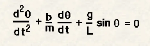
• g = gravity in m/s2,
• L = length of the pendulum in m,
• m = mass of the ball in kg,
• b=damping coefficient.

The way the pendulum moves depends on Newton's second law. When this law is written down, we get a second-order Ordinary Differential Equation that describes the position of the "ball" w.r.t time.

The objective of this program -

• The objective is to write a program that solves the following ODE. This ODE represents the equation of motion of a simple pendulum with damping

Errors occurred while programming -

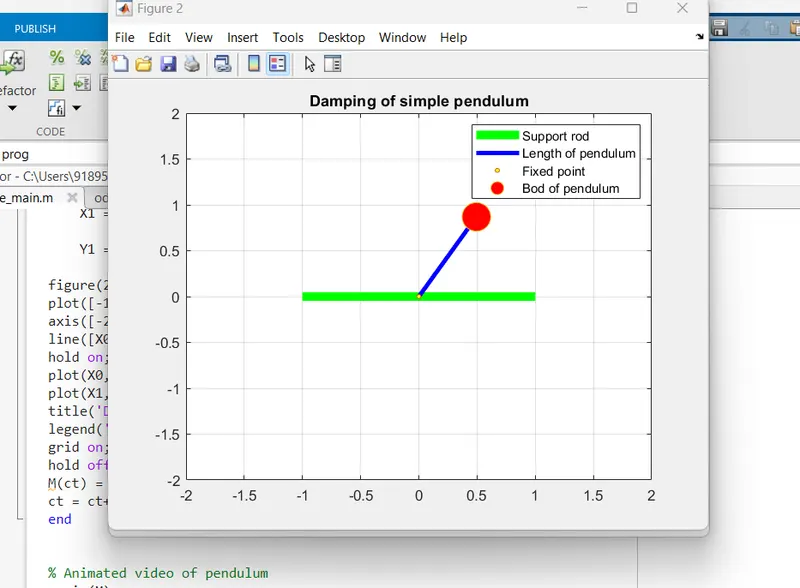
• Error1 - My pendulum is simulating in the opposite direction.

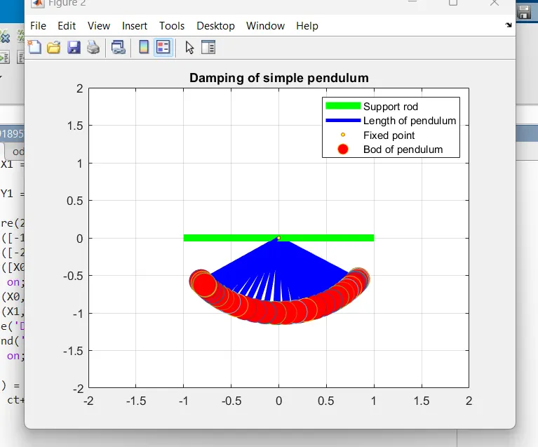
• Error 2 - traces of pendulum simulation are plotting on graph

Solution of errors -

• Error 1 - In error one I am getting the position of the pendulum in the opposite direction because I put the value of [Y1] positive after adding the [-] sign I get the accurate location of the pendulum.
• Error 2 - I am getting this error because I forgot to add the [Hold off] command after plotting.

Program to write ODE and animation of pendulum. -

clear all
close all
clc

% Inputs 

% g = gravity in m/s2,
% l = length of the pendulum in m,
% m = mass of the ball in kg,
% b = damping coefficient.

g = 9.81;
l = 1;
b = 0.05;
m = 1;

%initial condition 
theta_0 = [0;3];

%time points 
t_span = linspace(0,20,500);

% Solving ode 
[t,result] = ode45(@(t,theta) ode_func(t,theta,b,g,l,m),t_span,theta_0);


% Plotting of Simple plot of (Angular displacemnet) and (Anguler velocity)
plot(t,result(:,1),'linewidth',2,'Color','r')
hold on
plot(t,result(:,2),'linewidth',2,'Color','b')
legend('Angular displacemnet','Anguler velocity');
amplitude = result(:,1);
ct = 1;

% Creating loop for Simulation of pendulum 
for i = 1:length(amplitude)
    angle = amplitude(i);
    X0 = 0;
    Y0 = 0;
    X1 = l*sin(angle);
   
    Y1 = -l*cos(angle);

figure(2)
plot([-1 1],[0 0],'linewidth',6,'Color','g')
axis([-2 2 -2 2]);
line([X0 X1],[Y0 Y1],'linewidth',3,'Color','b')
hold on;
plot(X0,Y0,'O','MarkerSize',3,'MarkerFaceColor','y');
plot(X1,Y1,'O','MarkerSize',20,'MarkerFaceColor','r');
title('Damping of simple pendulum')
legend('Support rod','Length of pendulum','Fixed point','Bod of pendulum')
grid on;
hold off;
M(ct) = getframe(gcf);
ct = ct+1;
end


% Animated video of pendulum 
movie(M);
videofile = VideoWriter('Animation of simple pendulum','Uncompressed AVI');
open(videofile);
writeVideo(videofile,M);
close(videofile);

The function of this program -

function [dtheta_dt] = ode_func(t,theta,b,g,l,m)
theta1 = theta(1);
theta2 = theta(2);
dtheta1_dt = theta2;
dtheta2_dt = -(b/m)*theta2-(g/l)*sin(theta1);
dtheta_dt = [dtheta1_dt; dtheta2_dt];
end

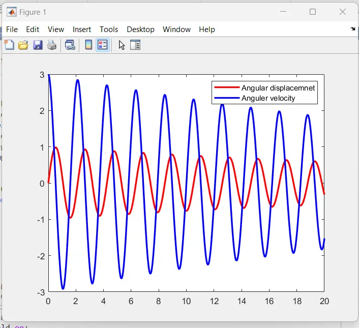
Graph of the motion between 0-20 sec, for angular displacement=0,angular velocity=3 rad/sec at time t=0 after this program -

Animated video of the pendulum -

https://youtu.be/n-uo2VXpdaE